fcmaes - a Python 3 gradient-free optimization library

This tutorial is about:

A typical machine learning hyperparameter tuning problem.
A comparison of common approaches, including Tree of Parzen Estimators and Bayesian Optimization, with fcmaes DE and CMA-ES.
How fcmaes algorithms improve as the evaluation budget grows.

Hyperparameter Tuning

How do we choose good parameter values for a learning algorithm? In machine learning, these parameters are called "hyperparameters". They control the learning process. Parameter optimization matters in many domains, but learning algorithms have a few specific properties:

The objective function is usually the mean square error of the prediction on the training data set.
Cross validation is expensive, but it usually supports parallel execution.
If cross validation already runs in parallel, the optimization algorithm itself does not need to be parallelized.
The optimization algorithm overhead is therefore less important.
Some parameters are discrete values, integers, or integer multiples of a real value.

In Python, four approaches are especially common:

Examples such as gear_train.py show that a discrete parameter can often be handled by mapping a real-valued parameter to a discrete one. That makes standard evolutionary real-valued optimizers such as CMA-ES, DE, and BITE applicable here. Even so, these methods are mostly ignored, apart from some research that uses Differential Evolution.

This tutorial looks at why that may be the case. We use a real-world example, House Price Prediction: "With 79 explanatory variables describing (almost) every aspect of residential homes in Ames, Iowa, this competition challenges you to predict the final price of each home."

The tutorial code house.py is based on the House Price Tutorial. We extended it with alternative hyperparameter tuning methods. To run the example, you need the house price data.

The original House Price Tutorial used only grid search to tune eight parameters of xgboost.XGBRegressor, one of the most widely used tools on kaggle. Only max_depth is truly discrete. The other parameters were discretized to make grid search faster. For a fair comparison we keep the same limits, but we use continuous values where possible.

Grid Search

# grid search

parameters_for_testing = {
    'colsample_bytree':[0.4,0.6,0.8],
    'gamma':[0,0.03,0.1,0.3],
    'min_child_weight':[1.5,6,10],
    'learning_rate':[0.1,0.07],
    'max_depth':[3,5],
    'n_estimators':[10000],
    'reg_alpha':[1e-5, 1e-2,  0.75],
    'reg_lambda':[1e-5, 1e-2, 0.45],
    'subsample':[0.6,0.95]
}

xgb_model = xgboost.XGBRegressor(learning_rate =0.1, n_estimators=1000, max_depth=5,
     min_child_weight=1, gamma=0, subsample=0.8, colsample_bytree=0.8, nthread=6, scale_pos_weight=1, seed=27)

gsearch = GridSearchCV(estimator = xgb_model, param_grid = parameters_for_testing,
                        n_jobs=6,iid=False, verbose=100, scoring='neg_mean_squared_error')
gsearch.fit(train_x, train_y)

#visualize the best couple of parameters
print (gsearch.best_params_)

The result is the following model, which is used later to generate the output:

best_xgb_model = xgboost.XGBRegressor(colsample_bytree=0.4,
                 gamma=0,
                 learning_rate=0.07,
                 max_depth=3,
                 min_child_weight=1.5,
                 n_estimators=10000,
                 reg_alpha=0.75,
                 reg_lambda=0.45,
                 subsample=0.6,
                 seed=42)

Results for the other methods

We tested on a single 16-core AMD 3950x CPU. For the CMA-ES tests we used the "parallel function evaluation" feature. That requires disabling parallelism in XGBRegressor by setting n_jobs=1. For all other tests, XGBRegressor parallelism was enabled.

We observed much better multi-core scaling with parallel function evaluation than with the internal parallelism of XGBRegressor. For CMA-ES, the number of evaluated function calls in a given time more than doubled. The tradeoff is higher memory consumption, because multiple parallel instances of XGBRegressor are kept alive.

Hyperband suggests that if you can double the number of evaluations, even random search may beat Bayesian Optimization. The results here go further. Even with the same number of evaluations, Bayesian Optimization and TPE are inferior to the evolutionary algorithms in this example. We did not find a good explanation for why standard evolutionary methods are still largely ignored in this area. Please contact me if you have an example where TPE or Bayesian Optimization outperforms standard evolutionary methods.

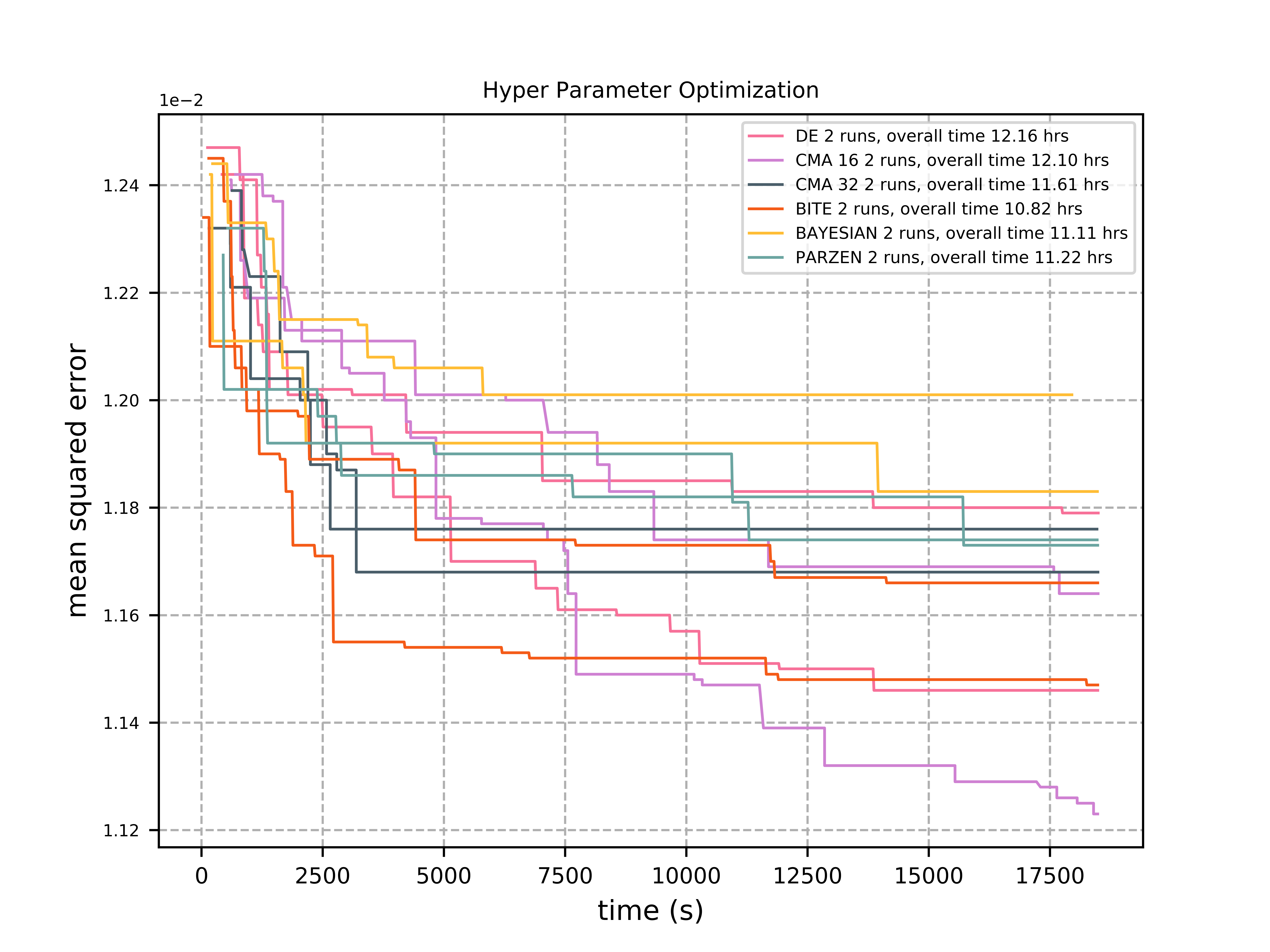
In the figure, CMA-16 means popsize=16, workers=16, and CMA-32 means popsize=32, workers-32. We observed sub-optimal scaling above 16 parallel function evaluations. That is not the case for parallel optimization runs. On this processor, 32 parallel optimizations are optimal. Here, however, XGBRegressor cross validation is too expensive, so parallel optimization does not make sense.

Objective function

To test the other methods, we first define a real-valued objective function. It computes neg_mean_squared_error by cross validation. We print the elapsed time, the best value found so far, and the number of evaluations used. mp.RawValue lets this work even when the objective function is called in parallel. For max_depth=int(X[4]), we map the real-valued parameter to an integer by truncating the decimal part.

# shared with all parallel processes
best_f = mp.RawValue(ct.c_double, -math.inf)
f_evals = mp.RawValue(ct.c_int, 0)
t0 = time.perf_counter()

# Optimization objective
def cv_score(X):
    X = X[0]
    score = cross_val_score(
            XGBRegressor(colsample_bytree=X[0],
                         gamma=X[1],
                         min_child_weight=X[2],
                         learning_rate=X[3],
                         max_depth=int(X[4]),
                         n_estimators=10000,
                         reg_alpha=X[5],
                         reg_lambda=X[6],
                         subsample=X[7],
                         #n_jobs=1 # required for cmaes with multiple workers
                         ),
                train_x, train_y, scoring='neg_mean_squared_error').mean()

    score = np.array(score)

    global f_evals
    f_evals.value += 1
    global best_f
    if best_f.value < score:
        best_f.value = score

    print("time = {0:.1f} y = {1:.5f} f(xmin) = {2:.5f} nfev = {3} {4}"
          .format(dtime(t0), score, best_f.value, f_evals.value, X))

    return score

Remark

Using mp.RawValue to share state between processes works only when subprocesses are forked, which is the default on Linux. Windows only supports spawning new processes, so there will be separate instances of best_f and f_evals if multiple workers are configured with fcmaes.cmaes or fcmaes.de. On Python 3.8, shared memory could be used instead, but we do not want to require Python 3.8 yet.

The mean squared error for the parameters found by grid search, [0.4, 0, 1.5, 0.07, 3, 0.75, 0.45, 0.6], is 0.01289. Next we see whether we can improve on that using

Bayesian Optimization

Instead of bounds, we define the feasible parameter values with the domain specification bds.

# Bayesian Optimization

from GPyOpt.methods import BayesianOptimization

bds = [
        {'name': 'colsample_bytree', 'type': 'continuous', 'domain': (0.4, 0.8)},
        {'name': 'gamma', 'type': 'continuous', 'domain': (0, 0.3)},
        {'name': 'min_child_weight', 'type': 'continuous', 'domain': (1.5, 10)},
        {'name': 'learning_rate', 'type': 'continuous', 'domain': (0.07, 0.1)},
        {'name': 'max_depth', 'type': 'discrete', 'domain': (3, 5)},
        {'name': 'reg_alpha', 'type': 'continuous', 'domain': (1e-5, 0.75)},
        {'name': 'reg_lambda', 'type': 'continuous', 'domain': (1e-5, 0.45)},
        {'name': 'subsample', 'type': 'continuous', 'domain': (0.6, 0.95)}]

optimizer = BayesianOptimization(f=cv_score,
                                 domain=bds,
                                 model_type='GP',
                                 acquisition_type ='EI',
                                 acquisition_jitter = 0.05,
                                 exact_feval=True,
                                 maximize=True)

optimizer.run_optimization(max_iter=20000)
y_bo = np.maximum.accumulate(-optimizer.Y).ravel()
print(f'Bayesian optimization neg. MSE = {y_bo[-1]:.2f}')

Tree of Parzen Estimators (TPE)

To support tree search, we "discretize" some of the parameters in the domain specification xgb_space.

# Parzen Tree Search

from hyperopt import fmin, hp, tpe, STATUS_OK

def obj_fmin(X):
    return {'loss': -np.asscalar(cv_score([X])), 'status': STATUS_OK }

xgb_space = [
        hp.quniform('colsample_bytree', 0.4, 0.8, 0.05),
        hp.quniform('gamma', 0, 0.3, 0.05),
        hp.quniform('min_child_weight', 1.5, 10, 0.5),
        hp.quniform('learning_rate', 0.07, 0.1, 0.05),
        hp.choice('max_depth', [3,4,5]),
        hp.uniform('reg_alpha', 1e-5, 0.75),
        hp.uniform('reg_lambda', 1e-5, 0.45),
        hp.uniform('subsample', 0.6, 0.95)]

best = fmin(fn = obj_fmin, space = xgb_space, algo = tpe.suggest,
                max_evals = 20000, verbose=False)

fcmaes Optimization Algorithms

For standard real-valued optimization algorithms, we define real bounds. Because we use max_depth=int(X[4]), the real-valued parameter is mapped to an integer by truncating the decimal part. This means the upper bound should be 6, so that max_depth=5 still has a corresponding real-valued interval of size 1.0. When cmaescpp.minimize uses multiple parallel workers, we have to disable parallelism in XGBRegressor by setting n_jobs=1.

This tutorial continues in delayed update tutorial where we focus on algorithms that support delayed optimization state updates.

# fcmaes optimization methods

from scipy.optimize import Bounds
from fcmaes import decpp, cmaescpp, bitecpp, de

bounds = Bounds([0.4, 0, 1.5, 0.07, 3, 1e-5, 1e-5, 0.6], [0.8, 0.3, 10, 0.1, 6, 0.75, 0.45, 0.95])

def obj_f(X):
    return -cv_score([X])

ret = bitecpp.minimize(obj_f, bounds, max_evaluations = 20000)

# for cmaescpp with multiple workers set n_jobs=1 in XGBRegressor

#ret = cmaescpp.minimize(obj_f, bounds, popsize=16, max_evaluations = 20000, workers=16)
#ret = cmaescpp.minimize(obj_f, bounds, popsize=32, max_evaluations = 20000, workers=32)
#ret = decpp.minimize(obj_f, 8, bounds, popsize=16, max_evaluations = 20000)

# delayed state update
#ret = cmaes.minimize(obj_f, bounds, popsize=16, max_evaluations = 20000,
#   					workers=32, delayed_update=True)

#ret = de.minimize(obj_f, bounds, popsize = 16, max_evaluations = 20000, workers=32)