fcmaes - a Python 3 gradient-free optimization library

Planning a 5G network

This tutorial

Shows how to plan a 5G network by optimizing the placement of sender stations to minimize their coverage radius / required energy.
Solves the p-center-problem where the region to cover is an irregular polygon containing irregularly shaped "holes".
Compares results of our approach to https://github.com/profyliu/p-center-problem .
See also Service.adoc, which handles a similar problem.

p-center-problem for irregular shapes with irregular holes

This tutorial is inspired by p-center-problem, which implements four different algorithms for this problem. See findrp.pdf for a description of the newest algorithm. The p-center problem places p facilities / sender stations so the whole region is covered. All senders are assumed to have the same power / range, and the goal is to minimize that range radius by relocating the p sender stations inside the area. The task becomes challenging when the coverage region contains "holes", because a sender cannot be placed inside a hole. It becomes even harder because the "holes" themselves do not need to be covered, and a good solution can use that fact to reduce the required range. We apply the BiteOpt optimization algorithm with parallel retry to make effective use of modern many-core CPUs.

Motivation

findrp.pdf states: "this is the most generic form (hence most difficult) among all known p-center problem variants". Here, "difficult" mainly refers to designing dedicated algorithms and proving their mathematical properties. That does not always mean a generic method is harder to apply or produces worse results.

Deep neural nets are a familiar example. They often solve problems where dedicated algorithms struggle, largely because they make good use of parallel computation on modern GPUs. CPU development has also moved toward parallelism, while many traditional algorithms are hard to adapt to it. Some optimization methods benefit from this trend more than others. Convex optimization often does. Evolutionary algorithms do as well because they evaluate populations of candidate solutions in parallel. In general, this trend favors generic algorithms over dedicated ones.

The question is whether the same is true for the p-center-problem for irregular shapes. The rest of this tutorial explores that.

General disadvantages of dedicated algorithms like the one described in findrp.pdf are:

Optimization can more easily get stuck in a local minimum if the solutions can change only locally but not globally.
It becomes more difficult to handle problem variations like adding noise, additional constraints or objectives.
It is harder to utilize parallelism.
It is more difficult to produce significantly different results performing multiple optimizations.

Their main advantage is often single threaded performance. But if the computation time is still feasible, a few seconds or minutes, then flexibility, ease of implementation, and solution quality often matter more. A significantly smaller range radius can mean much less sending power, see wireless-range-calculations. Note that the sending power scales logarithmically / grows exponentially. If your range radius is limited, you may need fewer sending stations instead. Compare that saving with the additional energy used by the optimizing CPU.

Results

For p=20, using 200000 fitness evaluations, the computation needs about 205 seconds and produces a maximal radius = 7.146 (see fcmaes_nd.p20.pdf). vorheur.py reaches radius = 8.667 (see vorheur_sol.p20.pdf). That is more than 21% improvement for the generic approach over the dedicated algorithm.

Using only 50000 fitness evaluations, the optimization finishes after 52 seconds and reaches radius = 7.57.

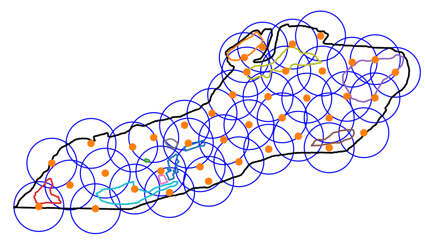
For p=40, the difference grows. vorheur.py achieves radius = 6.312, compared to radius = 5.117 for fcmaes, which is more than 23% improvement. fcmaes took 942 seconds here. The plots also show why: vorheur.py covers all holes, while fcmaes uses the fact that these do not need to be covered.

vorheur.py result for p=40

optimize.py result for p=40 showing the demand point grid

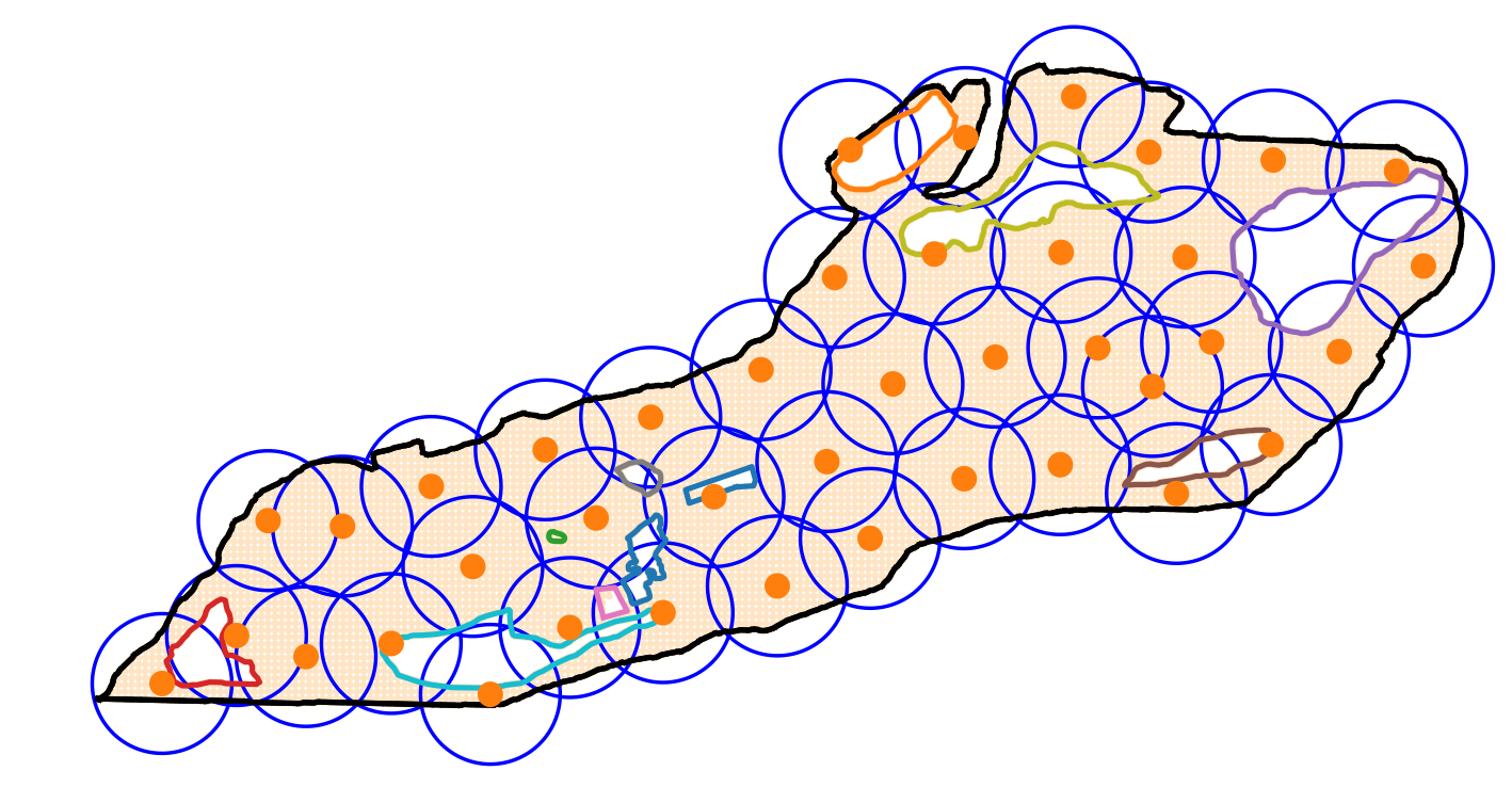
Note that the comparison is not completely fair. Because a demand point grid is used, there can be minor "coverage holes" where no demand point falls into that area. But since the grid uses a configured distance of 0.5, increasing the radius by at most 0.25 fills all "coverage holes".

Implementation

The complete code can be found at optimize.py.

The idea is:

Use all vertices of the outer polygon and all holes as demand points.
Add a grid of about 10000 demand points, filtered for feasibility: inside the outer polygon and outside the holes.
Use matplotlib.path.contains_points to determine if a point is valid.
Use numba to speed up the fitness calculation.
Utilize modern many-core CPUs, tested on the AMD 5950x 16 core CPU.

We convert the irregular coverage area with holes into a large grid of demand points. That turns the problem into a much simpler p-center variant, although we still have to keep the stations out of the "holes". To preserve accuracy, we use about 10000 demand points. At first glance this looks like a bad trade-off. For 40 sending stations, one fitness evaluation requires about 400.000 distance computations.

In practice it works well. If we keep most of the computation inside the CPU cache, avoid square roots by comparing squared distances, and use numba to compile the code with LLVM into a highly efficient executable, the evaluation is fast enough. A modern 16 core CPU like the AMD 5950x can execute about 15.000 fitness evaluations per second, each involving 400.000 distance computations, if 32 optimizations are performed in parallel. This number already includes the overhead of the optimizer itself.

The inner loop used for the fitness computation then looks like this:

    @njit(fastmath=True) # maximum of the minimal distances for all demand points
    def fitness_(facilities_x, facilities_y, demands):
        max_r = 0
        for i in range(len(demands)):
            min_r = 1E99
            for j in range(len(facilities_x)):
                dx = demands[i,0] - facilities_x[j]
                dy = demands[i,1] - facilities_y[j]
                # we use the square of the distance because it is faster to compute
                r = dx*dx + dy*dy
                if r < min_r: min_r = r
            if min_r > max_r: max_r = min_r
        return np.sqrt(max_r)

Never try this coding style with nested loops in plain Python. numba works well with numpy arrays, so this method takes the x- and y-coordinates of the sending stations / facilities as 1-dimensional arrays and the demand points as a 2-dimensional array. It returns the maximum of the minimal distances for each demand point. The square root is computed only once, for that maximum.

The objective function is then represented by a class Fitness initialized with

p, the number of stations/facilities,
corners, the coordinates of the vertices of the outer polygon,
holes_corners, the coordinates of the vertices of the holes, and
tolerance determining the grid spacing.

We use tolerance = 0.5 to limit the number of demand points in the grid to about 10000. The boundaries of the decision variables, which represent the station coordinates, are derived from the outer vertices (corners). The fitness function first checks for constraint violations by counting the number of stations outside the outer polygon or inside the holes. These get a huge penalty, 1E10 * violation_number. Only if there is no violation is the numba function fitness_ above called to determine the maximal demand-station distance.

    class Fitness():

        def __init__(self, p, corners, holes_corners, tolerance):
            self.p = p
            self.dim = self.p * 2
            cmax = np.amax(corners, axis=0)
            cmin = np.amin(corners, axis=0)
            lower = [cmin[0]]*p + [cmin[1]]*p
            upper = [cmax[0]]*p + [cmax[1]]*p
            self.generate_demands(tolerance, cmin, cmax, corners, holes_corners)
            self.bounds = Bounds(lower, upper)
 ...
        def fitness(self, x):
            facilities_x = x[:self.p]
            facilities_y = x[self.p:]
            facilities = [ [facilities_x[i], facilities_y[i]] for i in range(self.p)]
            penalty = 0
            for path in self.pathes: # penalty for facility in hole
                penalty += sum(path.contains_points(facilities))
            # penalty for facility outside outer
            penalty += sum(np.logical_not(self.path.contains_points(facilities)))
            if penalty > 0:
                return 1E10*penalty
            return fitness_(facilities_x, facilities_y, self.demands)

As demand points we use all polygon vertices, from the outer polygon and all holes, together with a demand grid spaced according to the tolerance parameter.

        def generate_demands(self, tolerance, cmin, cmax, corners, holes_corners):
            x = np.arange(cmin[0], cmax[0], tolerance)
            y = np.arange(cmin[1], cmax[1], tolerance)
            xs, ys = np.meshgrid(x, y)
            demands = np.vstack(list(zip(xs.ravel(), ys.ravel()))) # use grid demands
            path = mpltPath.Path(corners,closed=True)
            self.path = path
            self.pathes = []
            demands = demands[path.contains_points(demands)] # filter demands not in outer
            demands = np.concatenate((demands, corners))
            for hole_corners in holes_corners: # filter demands in holes
                path = mpltPath.Path(hole_corners, closed=True)
                demands = demands[np.logical_not(path.contains_points(demands))]
                demands = np.concatenate((demands, hole_corners))
                self.pathes.append(path)
            self.demands = demands

The grid points are filtered to exclude all points outside the outer polygon and inside the holes.

Designing the Fitness class is almost all we have to do when applying the fcmaes library here. There is no problem-specific algorithm design beyond the objective and constraints. Parallel optimization is performed using retry.minimize, and wrapper monitors the progress of all parallel executions.

The optimization driver is then:

    def optimize(fit, opt, num_retries = 32):
        ret = retry.minimize(wrapper(fit.fitness),
                                   fit.bounds, num_retries = num_retries,
                                   optimizer=opt, logger=logger())
        print("facility locations = ", fit.get_facilities(ret.x))
        print("value = ", ret.fun)
        return fit.get_facilities(ret.x), ret.fun

Next we have to choose a continuous optimizer. A good first choice is BiteOpt (Bite_cpp). In many cases, including this one, it performs very well. BiteOpt is a meta-algorithm that "learns" on the fly and adapts both its parameters and even its optimization method. If you can afford more optimization time, it can help to fine tune parameters such as popsize, the population size of the intermediate solutions it maintains.

   def run_optimize(corners, holes_corners, tolerance = 0.5, ndepots=20):
        fit = Fitness(ndepots, corners, holes_corners, tolerance)
        max_evaluations = 50000 # takes < 52 seconds on AMD 5950x
        opt = Bite_cpp(max_evaluations)
        # max_evaluations = 200000 # takes < 205 seconds on AMD 5950x
        # opt = Bite_cpp(max_evaluations, popsize=512)
        facilities, distance = optimize(fit, opt, num_retries = 32)
        plot("optimize", facilities, distance, ndepots, fit.demands)
        plot("optimize_nd", facilities, distance, ndepots, None)

Finally, we create a specific problem instance by parsing the kml files corresponding to the outer polygon and the holes:

    outer_file = 'belle_outer.kml'
    hole_files =  ['belle_botany2', 'belle_dock', 'belle_pavillion1', 'belle_pond1', 'belle_pond3', 'belle_pond5',
                    'belle_botany', 'belle_playground', 'belle_pond2', 'belle_pond4', 'belle_tennis_court']
    corners, holes_corners = parse_kml(outer_file, hole_files)
    run_optimize(corners, holes_corners)

Both the parsing and the plotting of the resulting solutions were taken almost without changes from the original repository https://github.com/profyliu/p-center-problem .

Conclusion

The p-center-problem for irregular shapes with irregular holes can be efficiently solved by dedicated algorithms, but the results do not seem to consider that the holes do not need to be covered.
For problem instances involving many stations / facilities, the generic approach using continuous optimization produces significantly better results.
The generic approach often requires more computing resources, which can be partly mitigated by parallelization and an efficient fitness implementation.
The BiteOpt algorithm in connection with parallel retry is a good choice for this problem.
The generic approach is well suited for 5G network design when the area to be covered is irregular and contains holes.