fcmaes - a Python 3 gradient-free optimization library

Optimization of a Variational Qubit

This tutorial starts with a very small quantum optimization problem. It then uses that example to compare optimizers and parallelization strategies in fcmaes.

It adapts Example-with-a-Single-Qubit-Variational-Form
It compares three fcmaes algorithms (DE, CMA-ES, and BiteOpt) with the IBM choice (COBYLA).
It tests different parallelization methods for optimization with the qasm_simulator from Qiskit.

The code for this part of the tutorial is here:

quant.py.

The same optimization ideas can also be transferred to a vendor-independent quantum infrastructure such as qcc.

Optimization of a VQE (Variational Quantum Eigensolver)

The second part asks whether the same lessons apply to a larger example: a VQE for the maxcut graph problem.

It adapts 06_examples_max_cut_and_tsp.html to test parallel optimization with both fcmaes and qiskit optimizers.
It compares results for different simulation backends.
It checks what changes when noise is added.

The code for this part of the tutorial is here:

maxcut.py.

How does a Quantum Computer work?

A quantum computer combines digital control with analog-like state evolution. If you want a broader introduction, see Quantum programming, the textbook, and this introduction. At a high level it works like this:

Conventional bits are transformed into qubits.
A quantum algorithm is a network of qubit gates executed on a simulator or a real quantum computer.
The resulting qubits are transformed back into conventional bits.

A qubit can be represented by a 3-dimensional unit vector. Qubit gates rotate this vector in different directions. You can use the colored buttons on the bloch sphere to see these operations directly. Control gates correlate multiple qubits. This correlation is called "entanglement". It means that a target qubit changes its probability and phase depending on a control qubit, so the qubits are no longer independent.

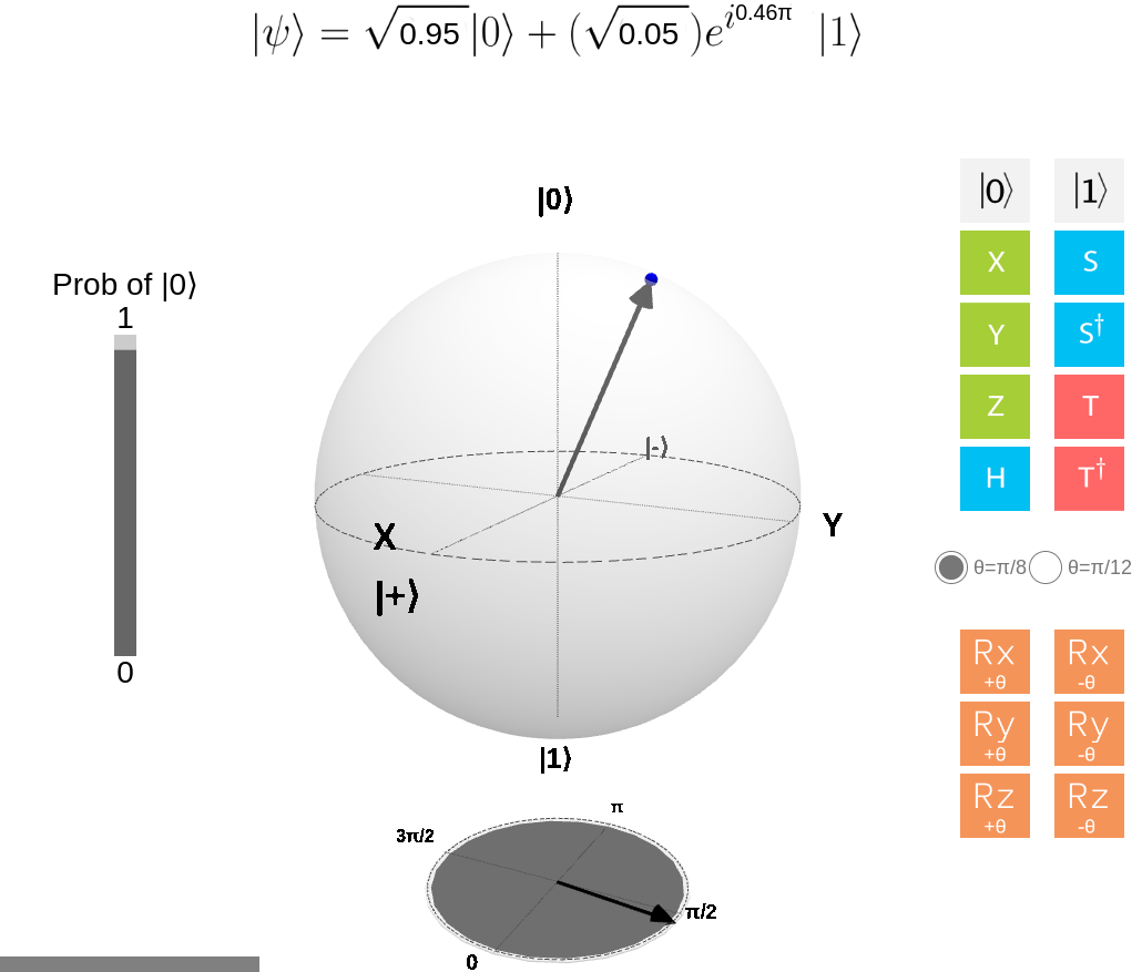
A qubit carries both a probability distribution and a phase. Only the probability part can be observed directly. When you measure a qubit, it collapses into a conventional bit according to that probability distribution.

The expressive power of a sequence of qubits is based on the following facts:

A single qubit corresponds to a continuous probability and phase.
N qubits represent 2^N probabilities, one for each bit combination they can collapse into.

How do we make sure that the final state means something useful after measurement? Techniques such as quantum Fourier transform and amplitude amplification use phase relationships to emphasize the desired bit combinations in the final probability distribution.

Quantum Optimization

Quantum optimization often uses a variational algorithm. The idea is to vary a parameterized quantum circuit until it gives a good approximation to the solution of an optimization problem. From the perspective of classical continuous optimization, this means that the fitness function is implemented by a parameterizable quantum algorithm. This is especially natural in physics, because the system being modeled is already quantum. See challenge of quantum optimization. Simulating real quantum effects is expensive, so in principle a real quantum device can replace that part of the fitness function.

There is a large body of work on the "quantum approximate optimization algorithm" (QAOA), because it can already be applied, at least in part, on today’s imperfect quantum computers. But https://journals.aps.org/prl/abstract/10.1103/PhysRevLett.127.120502 and https://www.nature.com/articles/s41467-018-07090-4 report "barren plateaus" and theoretical limits when QAOA is applied to other domains. There are theoretical limits in deep neural networks too, and that setting has a similar structure: a parameterized system sits between inputs and outputs. Even so, deep networks can work extremely well. The important point is that experience from optimizing neural networks does not transfer automatically to quantum circuits. In deep learning we can often get away with relatively simple methods derived from gradient descent. In the quantum setting that may not be enough. As we will see below, even a trivial 1-qubit circuit is not as easy to optimize as it looks.

Why is it still useful to optimize quantum algorithms with classical simulation? Current quantum hardware often restricts qubit connectivity in ways that do not match the circuit we want to build. A simulator lets us study the optimization problem today, instead of waiting for future hardware with more qubits and more flexible wiring.

Can optimization related to quantum algorithms be parallelized?

All qubit gates are rotations of a 3-dimensional unit vector. Some use fixed angles. Others expose rotation angles that become continuous decision variables for the optimizer. If the backend is a real quantum computer, parallelization currently makes little sense because compute time there is still expensive. That may change in the future, but not yet.

Development and test backends are different. They simulate quantum gates on conventional CPUs and GPUs, so parallelization can help. In this tutorial we use a concrete example to measure both runtime and solution quality when optimization is parallelized on a simulation backend. The single-qubit example is too small to say much about simulator scaling, so we first benchmark qiskit on a larger workload: 10 runs of an 8-36 qubit inverse Fourier transform (see gist). We use a 16 core AMD 5950x CPU, a mainstream many-core CPU at around 500 USD at the time of writing. On this CPU we can expect about:

factor 6-8 scaling for parallel objective function evaluation.
factor 12-16 scaling for parallel optimization runs.

As GPU we used an NVIDIA GTX 1660 Ti.

For both optimization-level parallelization modes we have to switch off simulator parallelism (no device='GPU', max_parallel_threads=1), so this only makes sense if the simulator itself scales worse:

aer_simulator_density_matrix cannot handle 18 or more qubits on our machine,
aer_simulator_statevector fails at 30 qbits (insufficient memory).

Table 1. Simulation benchmark - 10 runs of inverse fourier transform, time in sec
simulator	options	time 8 qbits	time 12 qbits	time 18 qbits	time 24 qbits	time 30 qbits	time 36 qbits
aer_simulator	none	0.90	2.11	3.43	28.25	1427.3	14.14
aer_simulator	max_parallel_threads=1	0.91	1.82	4.28	111.28	9035.0	12.46
aer_simulator	device='GPU'	0.87	1.56	3.45	19.7	cuda error	13.89
qasm_simulator	none	0.89	1.60	2.93	29.12	1434.6	14.38
qasm_simulator	max_parallel_threads=1	0.90	1.60	4.09	110.66	9028.2	13.02
qasm_simulator	device='GPU'	0.87	1.56	3.14	19.83	cuda error	14.49
aer_simulator_statevector	none	0.91	1.58	3.61	28.85	1430.8	-
aer_simulator_statevector	max_parallel_threads=1	0.89	1.6	3.88	110.4	9022.1	-
aer_simulator_statevector	device='GPU'	0.87	1.56	2.96	19.31	cuda error	-
aer_simulator_density_matrix	none	0.91	10.06	-	-	-	-
aer_simulator_density_matrix	max_parallel_threads=1	0.89	34.15	-	-	-	-
aer_simulator_density_matrix	device='GPU'	0.87	4.01	-	-	-	-

Summarizing the results:

For a small number of qbits (⇐ 18), aer_simulator, qasm_simulator, and aer_simulator_statevector do not scale much, neither with multithreading nor with a GPU.
For 8 qubits this is also true for aer_simulator_density_matrix; for 12 qubits it reaches a factor of 3.5 with multithreading and 8.5 with a GPU.
For 24 and 30 qubits, aer_simulator, qasm_simulator, and aer_simulator_statevector reach about factor 3.5 with multithreading and factor 5.5 with a GPU.
For 36 qubits, strangely, we again do not see significant scaling. Maybe another simulation method is used internally.

These results suggest that if we do not use aer_simulator_density_matrix and the circuit is relatively small (⇐ 18 qbits), we can switch off simulator parallelism and use optimization-level parallelism instead. For larger circuits we should benchmark the concrete circuit first.

Single Qubit Variational Form

The problem solved by Example-with-a-Single-Qubit-Variational-Form is close in spirit to ground-state energy estimation. It chooses parameters for a single-qubit variational form so that the output distribution matches a random target distribution as closely as possible. The complete example code is in quant.py.

The objective_function is only slightly adapted from the qiskit textbook. It uses qiskit operations and the qasm_simulator backend to measure the distance to the random target distribution target_distr.

Objective Function

def objective_function(params, target_distr):
    # Obtain a quantum circuit instance from the parameters
    qc = get_var_form(params)
    # Execute the quantum circuit to obtain the probability distribution associated with the current parameters
    t_qc = transpile(qc, backend)
    qobj = assemble(t_qc, shots=NUM_SHOTS)
    result = backend.run(qobj).result()
    # Obtain the counts for each measured state, and convert those counts into a probability vector
    output_distr = get_probability_distribution(result.get_counts(qc))
    # Calculate the cost as the distance between the output distribution and the target distribution
    cost = sum([np.abs(output_distr[i] - target_distr[i]) for i in range(2)])
    return cost

It is wrapped in a callable Fitness object that stores the target distribution.

class Fitness(object):

    def __init__(self, target_distr):
        self.target_distr = target_distr
        self.bounds = Bounds([0]*3, [2]*3)

    def __call__(self, x):
        return objective_function(x, self.target_distr)

Comparison of Different Optimization Algorithms

All optimizers are given the same random target distributions, generated in advance, so the results are comparable.

    # generate Fitness objects associated to random target distributions
    fits = [Fitness(random_target_distr()) for i in range(10)]
    opt_differential_evolution_loop(fits)
    opt_cmaes_loop(fits)
    opt_biteopt_loop(fits)
    opt_COBYLA_evolution_loop(fits)

All fcmaes optimizers are configured to use 16 parallel threads. COBYLA is single-threaded. If you have a modern many-core CPU, you can reproduce the results by executing quant.py. We used a 16 core AMD 5950x CPU and an NVIDIA GTX 1660 Ti GPU for our tests.

Read getting_started for Python environment setup. You need:

    pip install qiskit

pip install qiskit-aer-gpu (GPU support) is not required to execute quant.py, and it does not work on AMD GPUs.

COBYLA using no Parallelism

The COBYLA setup was taken from Example-with-a-Single-Qubit-Variational-Form and serves as a reference point. We increased maxiter to rule out the iteration limit as the main issue.

def opt_COBYLA_evolution_loop(fits):
    for fit in fits:
        params = np.random.rand(3)
        optimizer = COBYLA(maxiter=50000, tol=0.0001)
        ret = optimizer.minimize(fun=fit, x0=params)

COBYLA is fast and uses far fewer than maxiter iterations. The problem is solution quality. On this simple 3-dimensional problem, COBYLA is not reliable:

    COBYLA time 0.6 distance 0.004723912057785329
    COBYLA time 1.22 distance 0.09254840670649922
    COBYLA time 1.79 distance 0.5775480074342264
    COBYLA time 2.35 distance 1.1746999540117542
    COBYLA time 2.86 distance 0.2301463621426788
    COBYLA time 3.32 distance 0.043142750403738134
    COBYLA time 3.86 distance 0.15785308878979398
    COBYLA time 4.47 distance 0.015941335709322213
    COBYLA time 4.95 distance 0.015568947833576152
    COBYLA time 5.45 distance 1.2604080177937873

    COBYLA mean distance = 0.3572580782883162
    COBYLA std distance = 0.45984856126261725

This raises an obvious question: would you trust the same algorithm on a more complex quantum optimization problem? qiskit maps COBYLA to the scipy implementation. scipy offers more reliable alternatives such as differential evolution, but there is always a tradeoff between reliability and convergence speed. fcmaes tries to mitigate that tradeoff by supporting parallelism.

Differential Evolution using Parallel Fitness Evaluation

fcmaes offers a different variant of differential evolution than scipy. It is tuned for fast convergence and multiple parallel retries. In this case it is configured for parallel function evaluation instead (workers=16):

    def opt_differential_evolution_loop(fits):
        ...
        for fit in fits:
            ret = de.minimize(fit, 3, fit.bounds, max_evaluations = 1000,
                              stop_fitness = 0.00001, workers=16)
            ...

It uses all 1000 configured fitness evaluations. That makes it slower than COBYLA on this tiny problem, but much more reliable:

    de time 1.08 distance 7.608794221475312e-05
    de time 2.15 distance 5.159329350079567e-05
    de time 3.23 distance 0.00025199256577354556
    de time 4.31 distance 9.995401175424967e-05
    de time 5.38 distance 5.363785732115378e-05
    de time 6.45 distance 0.00025724959626183264
    de time 7.53 distance 5.30887897939869e-05
    de time 8.62 distance 0.00014133570932223227
    de time 9.71 distance 3.105216642390607e-05
    de time 10.81 distance 0.00020801779378730456

    de mean distance = 0.00012240097261537604
    de std distance = 8.258724841147236e-05

We did not use the alternative C++ implementation of DE that fcmaes also offers, because parallel function evaluation is slower there in this specific application context.

CMA-ES using Parallel Fitness Evaluation

The fcmaes CMA-ES implementation also supports parallel function evaluation, which we use here:

    def opt_differential_evolution_loop(fits):
        ...
        for fit in fits:
            ret = cmaes.minimize(fit, fit.bounds, input_sigma=0.7,
                        max_evaluations = 1000, stop_fitness = 0.00001, workers=16)            ...

The results are close to fcmaes-DE, but slightly worse:

    cmaes time 0.51 distance 0.026598245672092756
    cmaes time 1.55 distance 0.004407006710436312
    cmaes time 2.59 distance 7.25900467107854e-05
    cmaes time 3.65 distance 0.0001793522710383244
    cmaes time 4.69 distance 0.00016477295389366597
    cmaes time 5.78 distance 9.85274772162259e-05
    cmaes time 6.83 distance 0.00011994884350791102
    cmaes time 7.87 distance 5.438697928394909e-05
    cmaes time 8.92 distance 4.5451310954014446e-05
    cmaes time 9.98 distance 0.00014988796844872532

    cmaes mean distance = 0.003189017023358267
    cmaes std distance = 0.007907630855455892

BiteOpt using Parallel Optimization Retry

BiteOpt is written in C++ and does not support parallel function evaluation like the two algorithms above. It is a good choice in single-threaded mode or in the context of multiple parallel optimization retries. That trades some performance for higher reliability.

def opt_biteopt_loop(fits):
    ...
    for fit in fits:
        ret = retry.minimize(fit, fit.bounds, logger = None,
                              num_retries=16, optimizer=Bite_cpp(100), workers=16)
    ...

These results are worse than differential evolution on this example, but BiteOpt may be better for harder optimization problems or larger quantum algorithms. It is also a strong option when used single-threaded with multithreaded or GPU-based simulations. In that setting, multiple sequential retries may be needed to get a reliable result.

    bite time 1.96 distance 7.608794221475312e-05
    bite time 3.85 distance 0.0001484067064991823
    bite time 5.76 distance 0.00145199256577358
    bite time 7.65 distance 9.995401175424967e-05
    bite time 9.57 distance 0.0001463621426788242
    bite time 11.48 distance 5.724959626185466e-05
    bite time 13.38 distance 0.0002530887897940204
    bite time 15.23 distance 0.00014133570932223227
    bite time 17.18 distance 3.105216642390607e-05
    bite time 19.11 distance 0.0009919822062127437

    bite mean distance = 0.0003397511836935346
    bite std distance = 0.000456672806132943

Search for Weaknesses of Optimization Algorithms

Finally we use parallel optimization to search for weaknesses of COBYLA. The fitness function runs a COBYLA optimization and searches for a target distribution and an initial guess that maximize the final distance returned by COBYLA:

    def find_COBYLA_weakness():

        def fitness(x):
            params = x[:3] # use first three decision variables as guess for COBYLA
            target_distr =  x[3:] # use two decision variables as target
            ...
            fit = Fitness(target_distr)
            ret = COBYLA(maxiter=50000, tol=0.00001).minimize(fun=fit, x0=params)
            return -ret.fun # we maximize the distance

        bounds = Bounds([0]*5, [2]*3 + [1]*2)
        ret = de.minimize(wrapper(fitness), 5, bounds, max_evaluations = 300, workers=16)
        print("worst COBYLA distance = " +  str(ret.fun))

We get

0.61 16 26.0 -0.16048111250104818 [1.5150607763293302, 0.855535102710067, 0.9443911196710082, 0.44315944374947586, 0.5568405562505241]
0.71 19 27.0 -0.3451956010096087 [1.2667012355920217, 0.6074735090610092, 0.0, 0.5760978005048043, 0.4239021994951956]
0.72 20 28.0 -0.39053196482825997 [1.819039398258975, 0.5500857586958143, 0.473575221093664, 0.39823401758587, 0.6017659824141299]
0.74 21 28.0 -0.4871209992729757 [1.817252059960992, 0.0, 0.43090691832695105, 0.6197604996364878, 0.3802395003635122]
1.38 33 24.0 -1.5241888666705452 [2.0, 0.9968046393254453, 0.6468567010495877, 0.7675944333352724, 0.2324055666647275]
2.94 70 24.0 -1.7722 [2.0, 1.164716055769154, 0.8828197082450224, 1.0, 0.0]
5.14 117 23.0 -1.7860626205507981 [2.0, 1.260050169662025, 1.1363082378155278, 0.996531310275399, 0.003468689724600905]
7.27 163 22.0 -1.8356 [2.0, 1.5650815562087286, 0.6690050055417369, 1.0, 0.0]
8.69 197 23.0 -1.9714 [1.9104317884199735, 1.7238262098841646, 0.6395695514606753, 1.0, 0.0]
worst COBYLA distance = 1.9714

This confirms that COBYLA can return very poor results on this toy problem.

Summary

The COBYLA algorithm proposed in Example-with-a-Single-Qubit-Variational-Form is quite unreliable even on this 3-dimensional single-qubit optimization problem.
More reliable alternatives usually converge more slowly.
Parallel optimization or parallel fitness evaluation can offset part of that cost.
All three fcmaes algorithms tested here work reliably on the single-qubit variational form problem.
Differential Evolution with parallel fitness evaluation offers the best time / reliability compromise in this example.
For bigger quantum algorithms, qasm_simulator, aer_simulator_statevector, and aer_simulator work well with multithreading and GPU support switched off, so optimization-level parallelism can be used effectively.
BiteOpt with parallel optimization retry is a strong option for more complex quantum optimization tasks.
Differential Evolution with parallel function evaluation can also serve as a meta-optimizer to search for weaknesses in optimization algorithms.

VQE (Variational Quantum Eigensolver)

Let us see whether what we learned so far applies to a larger example: parameterizing a VQE for the maxcut graph problem. Whether maxcut itself should be solved this way is still debatable for two reasons:

Classical solvers have improved a lot and remain competitive.
Noise produced by quantum gates is still a real issue.

Even so, this problem is still a useful benchmark for VQE optimization, which matters in many other areas. While using 06_examples_max_cut_and_tsp.html as a basis, we ran into several qiskit refactorings, so a number of imports had to be changed.

Compare Different Optimizers

Suppose our task is to compare optimizers for the maxcut VQE. Preliminary tests showed that the fcmaes optimizers from the first section do not work well here. That leaves us with two practical options:

SPSA from qiskit.
CR-FM-NES (Fast Moving Natural Evolution Strategy for High-Dimensional Problems, see https://arxiv.org/abs/2201.11422) from fcmaes.

First we need to wrap CR-FM-NES as a qiskit optimizer so that qiskit’s VQE implementation can use it:

This is done in class fcmaes_Optimizer(optimizers.Optimizer) in maxcut.py. The wrapper is generic in two ways:

It can consume any fcmaes optimizer.
It has a parameter max_retries. If max_retries > 1, the fcmaes parallel optimization retry mechanism is applied. Parameter workers can also restrict the number of parallel workers.

We can also go the other way and wrap SPSA as an fcmaes algorithm:

    class fcmaes_SPSA(Optimizer):

        def __init__(self, maxiter=1000):
            Optimizer.__init__(self, maxiter, 'SPSA')
            self.opt = SPSA(maxiter=maxiter) # guessing

        def minimize(self, fun, bounds, guess=None, sdevs=None, rg=None, store=None):
            if guess is None: # necessary for parallel retry
                guess = np.random.uniform(bounds.lb, bounds.ub) if rg is None else \
                        rg.uniform(bounds.lb, bounds.ub)
            ret = self.opt.minimize(fun, guess, bounds=[t for t in zip(bounds.lb, bounds.ub)])
            return ret.x, ret.fun, ret.nfev

Now we can also execute SPSA in parallel by using a double wrapping with 12000 evaluations / 6000 iterations:

    optimizer = fcmaes_Optimizer(fcmaes_SPSA(6000), max_retries = 32)

Note that fcmaes parallel retry does not forward an initial guess x0, because varying the starting point improves diversity across runs. We handle that here by generating a random guess. Other parameters of minimize are:

sdevs is the initial step size used to narrow or widen the search performed by the optimizer. CMA-ES and CR-FM-NES use this parameter. Lowering it can improve the diversity of parallel retries.
rg is a random generator. It helps preserve diversity if multiple processes are involved.
store is used to maintain optimization results for statistical evaluation.

Experiments

You can reproduce the experiments by adapting and executing maxcut.py. You need fcmaes version 1.4.3 for these experiments (pip install fcmaes --upgrade).

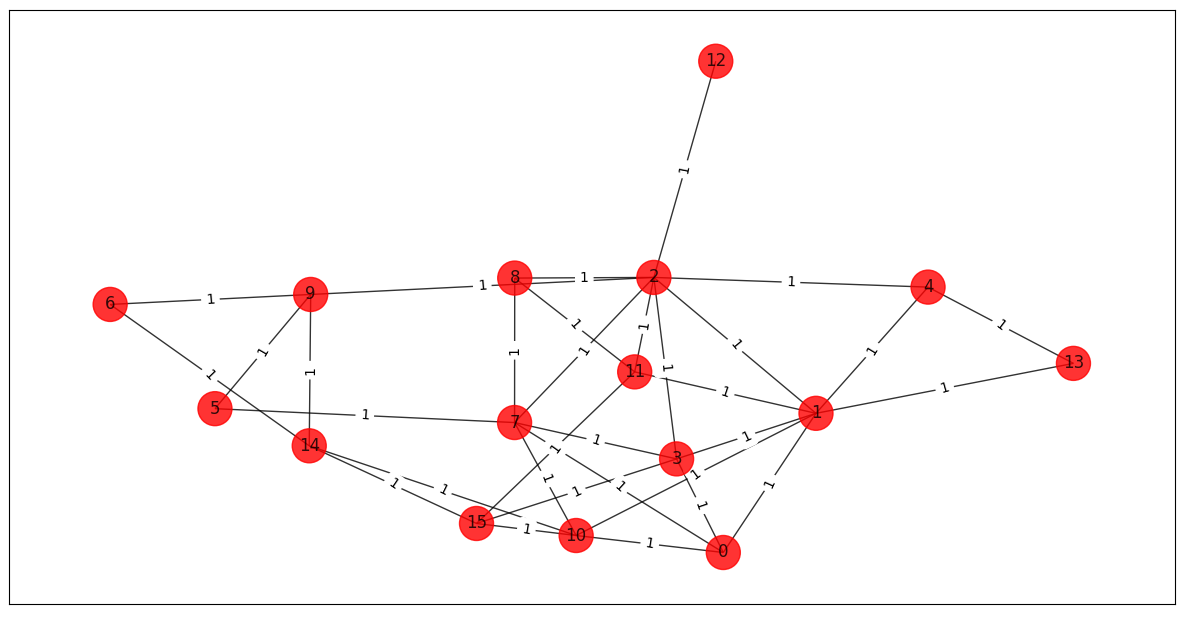
As in the original qiskit tutorial 06_examples_max_cut_and_tsp.html, we solve the maxcut graph problem, but we increase the graph size to n=16.

    G = nx.dense_gnm_random_graph(n, 2*n, seed=123)
    for (u, v) in G.edges():
        G.edges[u,v]['weight'] = 1

This generates a random 16-node graph with a fixed seed. With larger graphs the timing changes because processor cache size becomes a dominant limit. This graph leads to 96 continuous decision variables, which makes the optimization problem quite challenging. Even on modern CPUs, parallelization is needed if we want to run enough optimization attempts in reasonable time. All qiskit simulation parallelization happens in its C++ code, which is not publicly visible. It appears that qiskit relies on vector and matrix optimizations (BLAS) plus some other parallelization that becomes active for larger numbers of qubits or when noise is added.

All experiments were executed on a 16 core AMD 5950x CPU with 128 GB RAM on Linux Mint 20.3.

maxcut(SPSA(maxiter=6000), n, "aer_simulator")

Let us first check what qiskit-optimization offers out of the box. For this experiment we use qiskit’s default parallelization, which means temporarily removing with threadpoolctl.threadpool_limits(limits=1, user_api="blas"): and backend.set_options(max_parallel_threads=1) from the code. Without noise we get:

energy: -6.994140624999999
time: 661.4196128845215
max-cut objective: -22.994140625

This run takes more than 10 minutes and does not reach the optimum.

We see about 25% CPU load, which corresponds to roughly 4 cores on our 16 core CPU. How much does that parallelization actually help? Let us restore the with threadpoolctl.threadpool_limits(limits=1, user_api="blas"): and backend.set_options(max_parallel_threads=1) statements and rerun the experiment.

Now we see

This time only about half a core is used, and we get:

energy: -6.999023437500001
time: 544.7220184803009
max-cut objective: -22.9990234375

qiskit’s built-in parallelization seems to scale negatively here. Without it, the simulation is noticeably faster. What happens if we add noise?

maxcut(SPSA(maxiter=6000), n, "aer_simulator", add_noise=True)

With qiskit’s parallelization we see even higher CPU load:

and get

energy: -6.723632812500001
time: 1082.267616033554
max-cut objective: -22.72363281255

Noise slows things down even more. Without qiskit’s parallelization we get:

energy: -7.71875
time: 1006.533504486084
max-cut objective: -23.71875

Again qiskit’s parallelization hurts performance. The optimization results also differ between runs, so multiple retries are unavoidable. To compare algorithms in a meaningful way, we need a reasonable number of runs, and that quickly turns into many CPU-hours. Cloud machines are one option. There is also a cheaper one: parallelize at the optimization level.

During winter there is at least one benefit to qiskit’s parallelization: CPU temperature rises by about 10 degrees Celsius, so the machine can double as a room heater. Whether that compensates for negative scaling is another question. A better idea is to push parallelism into the optimizer itself. Before doing that, make sure nothing else is already parallelizing fitness evaluation.

First let us try parallel function evaluation. SPSA does not support it, so we switch to a fcmaes algorithm: CR-FM-NES (Fast Moving Natural Evolution Strategy for High-Dimensional Problems, see https://arxiv.org/abs/2201.11422). SPSA turned out to be better than the fcmaes optimizers from the first section, but CR-FM-NES is the relevant fcmaes comparison here.

maxcut(fcmaes_Optimizer(Crfmnes_cpp(12000, popsize=16, workers=16), use_wrapper=True), n, "aer_simulator")

Crfmnes_cpp uses the number of evaluations, not iterations, so we use 12000 instead of 6000 to configure the same number of function evaluations.

39.25 10000 255.0 -8.0 [-1.1634306611788974, -2.9237165862940446, ...]
energy: -8.0
time: 43.56654715538025
max-cut objective: -24.0

43 seconds means that, instead of negative scaling, we now get factor 544/43.5 = 12.5. Compared to qiskit parallelization, the factor is 661/43.5 = 15. Below we will check whether the good optimization result -8.0 was just luck.

With parameter use_wrapper=True we enable monitoring of the optimization, which produces output like:

24.68 7152 290.0 -8.000000000000002 [1.3432903811499826, -2.9505684864231103, ...]

This means:

24.68 : execution time in seconds.
7152 : number of fitness evaluations so far.
290.0 : number of fitness evaluations per second (eval/sec).
-8.0 : best fitness value so far.
[1.3432903811499826, -2.9505684864231103, …] : best solution vector so far.

Adding noise gives:

maxcut(fcmaes_Optimizer(Crfmnes_cpp(12000, popsize=16, workers=16), use_wrapper=True), n, "aer_simulator", add_noise=True)

energy: -7.744140624999998
time: 82.25768613815308
max-cut objective: -23.744140625

82.2 seconds, which is factor 1082/82.2 = 13.1 compared to SPSA with qiskit’s parallelization.

To compare SPSA and CR-FM-NES seriously, we need more runs. That means multi-start or retry for both optimizers. fcmaes can parallelize this for SPSA as well. But why use parallel retry for CR-FM-NES when it already supports parallel function evaluation? Because function-level parallelism adds overhead, and that overhead matters more when the individual tasks are short. An optimization run is much longer than a single fitness evaluation, so retry-level parallelism often scales better in total wall time. There is also a population-size constraint. Function-level parallelism cannot use more workers than the population size configured by the algorithm. Parallelizing full optimization runs does not have that restriction, so it can keep all CPU cores busy.

Use parallel fitness evaluation mode if you want a fast result.
Use parallel optimization retry if you want to test the reliability of an algorithm.

Let us first execute 32 SPSA optimization runs in parallel:

maxcut(fcmaes_Optimizer(fcmaes_SPSA(6000), max_retries = 32, use_wrapper=True, logger=logger()), n, "aer_simulator")

1065.9 360 32 384000 -8.000000 -7.28 0.80 [-8.0, -7.998, -7.998, -7.9971, -7.9971, -7.9951, -7.9951, -7.9951, -7.9941, -7.9932, -7.9922, -7.9912, -7.9883, -7.9883, -7.9883, -7.0, -7.0, -6.9971, -6.9971, -6.9971] ...
energy: -8.0
time: 1065.901137828827
max-cut objective: -24.0

Parameter logger=logger() is used to monitor the stream of results from the parallel runs:

1065.9 : execution time in seconds.
360 : number of fitness evaluations per second (eval/sec).
32 : number of finished optimization runs.
384000 : number of fitness calls.
-8.000000 : best fitness value so far.
-7.28 : mean value of all optimization results.
0.80 : standard deviation of all optimization results.
- [-8.0, -7.998, -7.998, -7.9971, -7.9971, -7.9951, …] list of the 20 best optimization results.

So for SPSA(6000) we get:

1066 seconds for 32 runs resulting in energy = [-8.0, -7.998, -7.998, -7.9971, -7.9971, -7.9951, -7.9951, -7.9951, -7.9941, -7.9932, -7.9922, -7.9912, -7.9883, -7.9883, -7.9883, -7.0, -7.0, -6.9971, -6.9971, -6.9971]
mean result: -7.28
standard deviation: 0.80

Note that we only see the best 20 runs here. Many of the 32 runs are very close to the absolute optimum of -8.0. Using parallel optimization we are faster by factor 32*661/1066 = 19.8 compared to serial restarts. That saves nearly 6 hours of CPU time.

For CR-FM-NES we get:

maxcut(fcmaes_Optimizer(Crfmnes_cpp(12000, popsize=16), max_retries = 16, use_wrapper=True, logger=logger()), n, "aer_simulator")

910.6 421 32 384000 -8.000000 -7.59 0.60 [-8.0, -8.0, -8.0, -8.0, -8.0, -8.0, -8.0, -8.0, -8.0, -7.999, -7.999, -7.999, -7.999, -7.998, -7.998, -7.9961, -7.9961, -7.9951, -7.9941, -7.9922] ...
energy: -8.000000000000004
time: 910.5991163253784
max-cut objective: -24.000000000000004

911 seconds for 32 runs resulting in energy = [-8.0, -8.0, -8.0, -8.0, -8.0, -8.0, -8.0, -8.0, -8.0, -7.999, -7.999, -7.999, -7.999, -7.998, -7.998, -7.9961, -7.9961, -7.9951, -7.9941, -7.9922]
mean result: -7.59
standard deviation: 0.60

This is faster and slightly better than SPSA. Using population size 24 slows things down slightly but improves the results further:

maxcut(fcmaes_Optimizer(Crfmnes_cpp(12000, popsize=24), max_retries = 16, use_wrapper=True, logger=logger()), n, "aer_simulator")

1110.17 345 32 384000 -8.000000 -7.69 0.58 [-8.0, -8.0, -8.0, -8.0, -8.0, -8.0, -8.0, -8.0, -8.0, -8.0, -8.0, -8.0, -8.0, -8.0, -8.0, -8.0, -8.0, -8.0, -8.0, -8.0]
energy: -8.000000000000004
time: 1110.1752026081085
max-cut objective: -24.000000000000004

1110 seconds for 32 runs resulting in energy = [-8.0, -8.0, -8.0, -8.0, -8.0, -8.0, -8.0, -8.0, -8.0, -8.0, -8.0, -8.0, -8.0, -8.0, -8.0, -8.0, -8.0, -8.0, -8.0, -8.0]
mean result: -7.69
standard deviation: 0.58

What about noise? Let us execute 32 SPSA optimization runs in parallel:

maxcut(fcmaes_Optimizer(fcmaes_SPSA(6000), max_retries = 32, use_wrapper=True, logger=logger()), n, "aer_simulator", add_noise=True)

1751.71 219 32 384000 -7.823242 -7.25 0.59 [-7.8232, -7.7383, -7.7236, -7.7158, -7.7061, -7.7051, -7.7041, -7.6934, -7.6846, -7.6777, -7.666, -7.6465, -7.6416, -7.6416, -7.6309, -7.6279, -7.6182, -7.6113, -7.6035, -7.5869]...
energy: -7.8232421875
time: 1751.7082085609436
max-cut objective: -23.8232421875

1752 seconds for 32 runs resulting in energy = [-7.8232, -7.7383, -7.7236, -7.7158, -7.7061, -7.7051, -7.7041, -7.6934, -7.6846, -7.6777, -7.666, -7.6465, -7.6416, -7.6416, -7.6309, -7.6279, -7.6182, -7.6113, -7.6035, -7.5869]
mean result: -7.25
standard deviation: 0.59

We need 1752 seconds for 32 runs, which means factor 1082*32/1752 = 19.8 compared to qiskit’s parallelization.

maxcut(fcmaes_Optimizer(Crfmnes_cpp(12000, popsize=16), max_retries = 32, use_wrapper=True, logger=logger()), n, "aer_simulator", add_noise=True)

1646.53 233 32 384000 -7.871094 -7.39 0.59 [-7.8711, -7.8564, -7.8555, -7.8496, -7.8496, -7.8486, -7.8193, -7.8008, -7.7969, -7.7578, -7.75, -7.749, -7.7402, -7.7363, -7.7363, -7.7314, -7.7285, -7.7256, -7.71, -7.6982] ...
energy: -7.871093749999998
time: 1646.533742904663
max-cut objective: -23.87109375

1647 seconds for 32 runs resulting in energy = [-7.8711, -7.8564, -7.8555, -7.8496, -7.8496, -7.8486, -7.8193, -7.8008, -7.7969, -7.7578, -7.75, -7.749, -7.7402, -7.7363, -7.7363, -7.7314, -7.7285, -7.7256, -7.71, -7.6982]
mean result: -7.39
standard deviation: 0.59

This is slightly faster and marginally better than SPSA. With noise, population size 24 does not improve things:

maxcut(fcmaes_Optimizer(Crfmnes_cpp(12000, popsize=24), max_retries = 32, use_wrapper=True, logger=logger()), n, "aer_simulator", add_noise=True)

1707.94 224 32 384000 -7.863281 -7.30 0.59 [-7.8633, -7.8418, -7.8271, -7.8018, -7.7979, -7.7529, -7.7441, -7.7324, -7.7295, -7.7246, -7.7236, -7.7031, -7.7002, -7.6982, -7.6875, -7.6836, -7.6807, -7.6572, -7.6475, -6.8662]
energy: -7.863281249999998
time: 1707.9386677742004
max-cut objective: -23.86328125

1708 seconds for 32 runs resulting in energy = [-7.8633, -7.8418, -7.8271, -7.8018, -7.7979, -7.7529, -7.7441, -7.7324, -7.7295, -7.7246, -7.7236, -7.7031, -7.7002, -7.6982, -7.6875, -7.6836, -7.6807, -7.6572, -7.6475, -6.8662]
mean result: -7.30
standard deviation: 0.59

Exercises

Test qasm_simulator with and without noise.
Try other graph sizes or seeds.

Summary

SPSA is an excellent algorithm for VQE optimization, especially if noise is involved.
CR-FM-NES (Fast Moving Natural Evolution Strategy for High-Dimensional Problems, see https://arxiv.org/abs/2201.11422) is a good alternative that may have advantages for more complex VQEs.
Both can be parallelized with fcmaes parallel restart/retry and show very good scaling.
With parallel function evaluation, CR-FM-NES is much faster than SPSA.
Maxcut parallelization scales best for qasm_simulator and aer_simulator, but fitness evaluation and quantum circuit simulation should be kept single-threaded.
Avoid the "room heater": do not run VQE circuit simulation multi-threaded until you have verified that it improves performance on your CPU. At least during summer time.