

Optimization with Constraints
This tutorial is about:
-
how to use a weighted-sum penalty approach for constraints in single-objective optimization.
-
how to apply this approach to a space mission design problem.
Not all optimization problems are box-constrained. Many also contain equality or inequality constraints. In this tutorial, we use a real example to show how such a problem can be converted into a box-constrained one. We also look at the drawbacks of that conversion. Finally, we show how dedicated constrained optimizers can be applied directly.
As an alternative, the fcmaes multi-objective MODE optimizer supports explicit constraints. These constraints are prioritized and weighted automatically. You can also apply MODE to a single-objective problem if you want to use that mechanism.
Fly to near earth asteroid K14Y00D
We use pykep example 11, which is based on lt_margo
This problem models a low-thrust interplanetary trajectory from Earth to the near-Earth asteroid "K14Y00D".
It was developed for the European Space Agency interplanetary cubesat M-ARGO study.
See CubeSat and to NEA
for more details. If you want to reproduce the experiments, install the dependencies with pip install pygmo and pip install pykep.
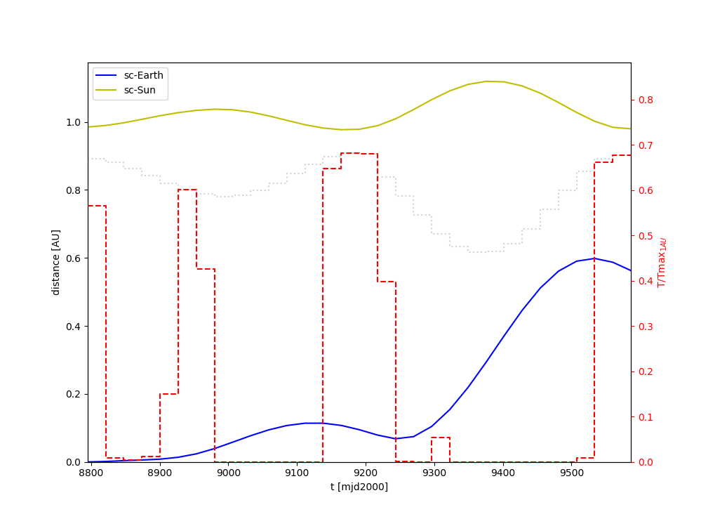
The trajectory is split into 30 equal segments. Each segment has its own maximum thrust, which depends on the distance from the Sun. A Taylor integrator propagates position, velocity, and mass numerically. The Taylor integrator is efficient, but each objective function evaluation is still expensive.
This problem is quite different from the GYM problems discussed in GYM results:
-
Example 11 has 93 dimensions, but it is still much easier than the GYM problems because it covers only a single segmented transfer. The GYM problems span multiple transfers and visits to many planets. They have lower dimensionality because they use only one segment per transfer.
-
The combination of high dimensionality and moderate difficulty has an important consequence: coordinated retry does not help much here. Instead, we need dedicated constrained optimizers, or pure CMA-ES with more evaluations per run and a smaller population size.
Objective Function
The basic idea is simple. We propagate 15 segments forward from the start and 15 segments backward from the target. Both trajectories should "meet" in the middle. This creates equality constraints for the mismatch in position, velocity, and mass. Each segment has its own thrust values. These values are computed from the argument vector and depend on the distance from the Sun, see L287
Since Example 11 does not include Earth gravity (earth_gravity=False), all inequality constraints come from the maximum thrust in each segment.
Thrust is represented as (x,y,z) vectors. Each component is box-constrained, but that is not enough. We also need inequality constraints to limit the total thrust, which is given by the norm of the thrust vector.
This leads to an important observation:
-
Sometimes inequality constraints can be converted into box constraints. In this case, we could represent each three-dimensional thrust vector in polar coordinates: two angles plus the norm. Those values could then be box-constrained.
Solving Example 11
Since the problem is defined as a PYGMO2 user-defined problem, it can be solved with PYGMO/PAGMO optimizers, as the Example 11 code shows:
    ...
    algo = algo_factory("snopt7")
    udp = add_gradient(pk.trajopt.lt_margo(
    prob = pg.problem(udp)
    prob.c_tol = [1e-5] * prob.get_nc()
    pop = pg.population(prob, 1)
    pop = algo.evolve(pop)
    print("Feasible?:", prob.feasibility_x(pop.champion_x))
    ...
In fact, PYGMO forwards the problem to the commercial SNOPT solver.
Open-source optimizers are also supported. If snopt7 is not available, we can switch easily:
    ...
    algo = algo_factory("slsqp")
    algo.set_verbosity(0)
    ...
        earth_gravity=False),
        with_grad=True
Now the NLopt slsqp algorithm is used instead. Let us try a serial loop first:
from fcmaes.optimizer import dtime

def test_loop(prob, algo):
    t0 = time.perf_counter()
    while True:
        pop = pg.population(prob, 1)
        pop = algo.evolve(pop)
        print('time', dtime(t0), 'champion_f', pop.champion_f[0], "Feasible?:",
              prob.feasibility_x(pop.champion_x))
resulting in:
time 72.34 champion_f -18.78035820300855 Feasible?: True
time 143.16 champion_f -18.85317527444599 Feasible?: True
time 206.46 champion_f -18.857317774033927 Feasible?: True
time 290.88 champion_f -18.237459651485377 Feasible?: True
time 371.64 champion_f -18.261442245473454 Feasible?: False
time 440.46 champion_f -18.24324031526028 Feasible?: True
time 525.19 champion_f -18.097314671335102 Feasible?: False
time 596.36 champion_f -18.791981422166668 Feasible?: True
time 601.63 champion_f -6.304079168374591 Feasible?: False
time 679.41 champion_f -18.03371887092075 Feasible?: False
time 682.53 champion_f -14.166934956585262 Feasible?: False
The results are quite inconsistent. We even get many infeasible solutions.
A serial loop is not a good way to tackle this problem. PYGMO provides a parallel execution model called archipelago:
Parallelization using PYGMO archipelago
def test_arch(prob, algo):
    I = mp.cpu_count()
    archi = pg.archipelago(n=I, algo = algo, prob = prob, pop_size=1)
    t0 = time.perf_counter()
    while True:
        archi.evolve()
        archi.wait()
        best = math.inf
        x = []
        for il in archi:
            pop = il.get_population()
            fs = pop.get_f();
            xs = pop.get_x();
            for i in range(len(fs)):
                if fs[i][0] < best:
                    best = fs[i][0]
                    x = xs[i]
        print('time', dtime(t0), 'champion_f', best, "Feasible?:",
              prob.feasibility_x(x))
All 16 cores of the 3950x are busy, and we get:
time 135.98 champion_f -18.857680581263764 Feasible?: True
time 261.04 champion_f -18.859695980942995 Feasible?: True
time 385.02 champion_f -18.859897566652382 Feasible?: True
time 509.38 champion_f -18.85990086555996 Feasible?: True
Using pg.archipelago with a non-population-based algorithm is unusual, but it works as intended.
The results become much more consistent, and we can run about 20 times more optimizations than with the serial loop.
In our case, mp.cpu_count() = 32, so we performed 32*4 = 128 optimizations in 509 seconds.
Applying fcmaes retry to PAGMO problems and algorithms
Next, let us see what fcmaes parallel retry can do. fcmaes provides pygmoretry specifically for PYGMO2 problems and algorithms.
A normal wrapper would not work because fcmaes usually expects the objective function to return a single fitness value, not a vector with constraints or multiple objectives. pygmoretry does not work with fcmaes optimizers themselves. Its purpose is to provide a simple parallel retry mechanism for constrained or multi-objective PYGMO problems.
    from fcmaes import pygmoretry
    from fcmaes.optimizer import logger
    ret = pygmoretry.minimize(prob, algo, num_retries = 640,
                    logger = logger())
    print(ret.fun, ret.nfev, ret.x)
results in:
98.6 21 37 2102 -18.782321 ...
99.01 42 38 4204 -18.795005 ...
99.98 63 39 6306 -18.823922 ...
101.4 82 40 8408 -18.858432 ...
...
485.77 372 174 180927 -18.858432 -18.69 0.19 ...
This time we complete 174 optimizations in 485 seconds. The scaling is better than with pg.archipelago.
The speedup is about a factor of 28, which is quite good for 16 cores and 32 logical CPUs.
After 101 seconds we already find a good solution with fitness -18.8584.
Possible reasons why pg.archipelago scales less well are:
-
We did not find documentation showing how to force the archipelago to use fork_island instead of thread_island.
fcmaesuses Python multiprocessing, which creates separate processes. -
fcmaesdoes not require workers to wait for each other as inarchi.wait(). All processes run independent loops and synchronize through shared memory. If individual optimizations take different amounts of time, there is no global waiting point.
How to convert constraints into penalties?
Next, let us see whether we can remove the explicit constraints. The idea is to replace them with a penalty term. PYGMO2 provides a special class for this, unconstrain, but let us implement it ourselves.
In constraint scaling, the position, velocity, and mass mismatches are already scaled in a consistent way:
-
using AU, the Earth-Sun distance, for the position mismatch
-
using Earth velocity for the velocity mismatch
-
using start mass for the mass mismatch
In general, it is a good idea to make different mismatches dimensionless.
from fcmaes import retry
from fcmaes.optimizer import logger, Cma_cpp

def penalty(val, prob):
    c_tol = prob.c_tol
    nec = prob.get_nec()
    nc = prob.get_nc()
    peneq = np.sum([abs(val[i+1])+1 for i in range(nec) if abs(val[i+1]) > c_tol[i]])
    peniq = np.sum([val[i+1]+1 for i in range(nec, nc) if val[i+1] > c_tol[i]])
    return 20*peneq + 20*peniq

class margo_problem:

    def __init__(self, udp):
        self.prob = pg.problem(udp)
        self.prob.c_tol = [1e-5] * self.prob.get_nc()
        self.name = self.prob.get_name()
        self.fun = self.fitness
        lb, ub = self.prob.get_bounds()
        self.bounds = Bounds(lb, ub)

    def fitness(self,X):
        val = self.prob.fitness(X)
        return val[0] + penalty(val, self.prob)

    def guess(self):
        return np.random.uniform(self.bounds.lb, self.bounds.ub)

def test_penalty(udp):
    mprob = margo_problem(udp)
    ret = retry.minimize(mprob.fitness, bounds=mprob.bounds,
                             optimizer=Cma_cpp(300000, popsize=13),
                             num_retries = 640, logger = logger())
Note that we add a kind of "mini death" penalty for constraint violations. This makes the objective function non-smooth, which is not a problem for the fcmaes optimizers.
We get:
183.97 1630 32 300002 1.284878
184.51 4877 34 900006 1.278997
185.53 16169 41 3000020 -18.678094
187.69 27172 48 5100034 -18.828764
190.06 31569 51 6000040 -18.853587
We find a solution with score -18.85358 in 190 seconds. That is not a bad result, but CMA-ES is neither as fast nor as reliable as NLopt slsqp.
Advantages of the penalty approach using CMA-ES:
-
We do not need to work with gradients. gradient_sparsity is not trivial to define.
-
The objective function can be non-smooth and does not need to be differentiable.
-
We can apply coordinated retry, which may be useful for harder optimization problems.
Problems with the penalty approach using CMA-ES:
-
How should we choose the weights in
return 20*peneq + 20*peniq? If they are too low, we get infeasible results. If they are too high, they can "disturb" the optimization process. -
The same applies to the CMA-ES parameters.
optimizer=Cma_cpp(300000, popsize=13)works well here, but other problems may need different settings. -
Can be slower and less reliable than a derivative based optimizer for specific problems.