fcmaes - a Python 3 gradient-free optimization library

Optimization of multi-objective problems using weighted sums

The code for this tutorial is at moexamples.py and uses moretry.py.

This tutorial shows:

How fcmaes single-objective optimizers, combined with a specialized parallel retry implementation, can be used to approximate the Pareto front of multi-objective problems.
Why strong results on easy benchmark problems, especially problems that random sampling can solve, do not predict performance on real-world problems.
How the weighted-sum approach can be used to compute a Pareto front while also parallelizing function evaluations.
Why standard algorithms such as NGSAII, when used without parallelization, can be several orders of magnitude slower than fcmaes multi-objective parallel retry on real-world problems. Parallel scaling matters, but it is only part of the explanation.

For real-world problems, the Pareto front is not always the final target. Assume our algorithm returns good solutions, including some that are only slightly dominated:

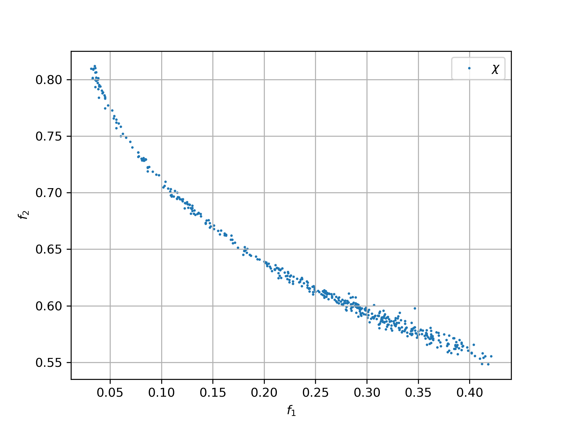
all .rw top trumps biobj f2i5d128 4k512 de cpp

In that case, computing the Pareto front immediately may be a bad idea:

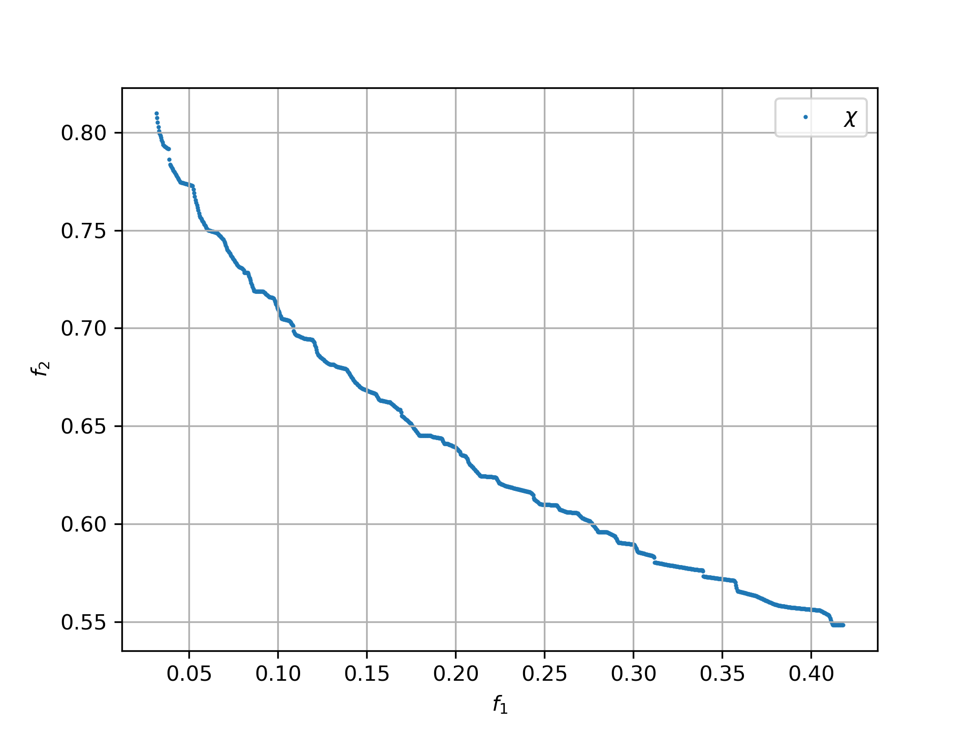
front .rw top trumps biobj f2i5d128 4k512 de cpp

There are several reasons:

Optimization is usually based on a slightly inaccurate model.
The model may be a surrogate chosen for fast evaluation.
Some very expensive objectives or constraints may have been left out.
Constraints may have changed after an optimization run with costly simulations has finished.

With the first result set, you can reevaluate the limited number of candidate solutions using a more accurate or updated model. Only then should you compute the Pareto front. A solution that was slightly dominated at first may become non-dominated after reevaluation.

UPDATE

fcmaes now includes a dedicated multi-objective algorithm, MO-DE, which also supports constraints. Try that first, especially for fitness functions with expensive evaluations. In that setting, MO-DE with parallel function evaluation is superior to moretry.py using parallel retry of single-objective algorithms. Test its parameters nsga_update and pareto_update to see which variant fits your problem best. If your problem is mixed-integer, do not forget to specify the ints parameter.

Experiments with artificial benchmark functions

fcmaes does not rely on a dedicated multi-objective algorithm here. Instead, it runs single-objective optimizers in parallel and applies random weighted sums. This often works surprisingly well, especially when the alternative is a single-threaded multi-objective algorithm. As we will see later, for many real-world multi-objective problems from space-flight planning with multiple gravity assists, this is the only approach here that delivers useful results in a reasonable time.

We start with artificial multi-objective benchmark functions from deap-tests. See MOBOpt for a description of these functions. As in that paper, we use the well-known benchmark functions Schaffer, Fonseca, Poloni, and ZDT1.

class zdt1:

    def __init__(self, dim):
        self.fun = db.zdt1
        self.bounds = Bounds([0]*dim, [1]*dim)
        self.weight_bounds = Bounds([0.01, 0.01], [1, 1])
        self.name = 'zdt1(' + str(dim) + ')'

class schaffer:

    def __init__(self, dim):
        self.fun = db.schaffer_mo
        self.bounds = Bounds([-1000]*dim, [1000]*dim)
        self.weight_bounds = Bounds([0.01, 0.01], [1, 1])
        self.name = 'schaffer(' + str(dim) + ')'

class poloni:

    def __init__(self, dim):
        self.fun = db.poloni
        self.bounds = Bounds([-math.pi]*dim, [math.pi]*dim)
        self.weight_bounds = Bounds([0.01, 0.01], [1, 1])
        self.name = 'poloni(' + str(dim) + ')'

class fonseca:

    def __init__(self, dim):
        self.fun = db.fonseca
        self.bounds = Bounds([-4]*dim, [4]*dim)
        self.weight_bounds = Bounds([0.01, 0.01], [1, 1])
        self.name = 'fonseca(' + str(dim) + ')'

The fcmaes library provides convenience functions for testing parallelized algorithms. They generate a detailed log file and a diagram that shows progress over time or the resulting Pareto front:

from fcmaes import moretry

def minimize_plot(problem, opt, name, exp = 2.0, num_retries = 1024, value_limits=None):
    moretry.minimize_plot(problem.name + '_' + name, opt,
                          problem.fun, problem.bounds, problem.weight_bounds,
                          num_retries = num_retries, exp = exp, value_limits = value_limits)

def adv_minimize_plot(problem, opt, name, value_limit = math.inf, num_retries = 10240):
    moretry.adv_minimize_plot(problem.name + '_' + name, opt,
                              problem.fun, problem.bounds, value_limit = value_limit,
                              num_retries = num_retries)

First, let us check random search with 1024 retries and 50000 evaluations per retry:

mo_retry_plot(zdt1(20), random_search(), '_random')
mo_retry_plot(schaffer(20), random_search(), '_random')
mo_retry_plot(poloni(20), random_search(), '_random', exp=1.0)
mo_retry_plot(fonseca(20), random_search(), '_random', exp=3.0)

Fonseca function random search, dim = 20, 1024 retries, 50000 evaluations:

Poloni function random search, dim = 20, 1024 retries, 50000 evaluations:

Python is surprisingly fast at converting these results into a Pareto front showing all non-dominated solutions:

Fonseca function, random search, dim = 20, 1024 retries, 50000 evaluations, pareto front:

Poloni function, random search, dim = 20, 1024 retries, 50000 evaluations, pareto front:

Now let us try two more benchmark problems:

Schaffer function, random search, dim = 20, 1024 retries, 50000 evaluations:

Pareto front:

ZDT1 function, random search, dim = 20, 1024 retries, 50000 evaluations:

Pareto front:

The ZDT1 result is not what we expected. Maybe a better optimizer helps:

ZDT1 function, de-cma sequence, dim = 20, 1024 retries, 50000 evaluations:

Pareto front:

What do we learn from this? For most artificial problems, no sophisticated optimizer is needed. Random search is often enough. These benchmark functions are designed to expose flaws in multi-objective algorithms. They do not resemble typical real-world problems. You should not use them to predict real-world performance. That is why we now switch to a more realistic case.

Real World Multi Objective Scenario

Suppose we work at NASA and need to plan the Cassini mission to Saturn. Fortunately, our colleagues at ESA prepared a useful Cassini model that we can adapt into a multi-objective fitness function. Our boss says the overall mission time should be < 2000 days. He leaves for a planning meeting in a few hours, and we need to show him why that target is unrealistic. To do that, we need the tradeoff between fuel consumption and mission time. In other words, we need the Pareto front for two competing objectives. We do not have time for a supercomputer. We only have a fast 16-core desktop (AMD 5950x).

We import ESA’s single-objective Cassini fitness function, which computes the overall delta velocity and therefore roughly the fuel consumption. The second objective, travel time, is easy to derive from the input arguments.

from fcmaes.astro import Cassini1

class cassini1_mo:

    def __init__(self):
        self.base = Cassini1()
        self.bounds = self.base.bounds
        self.weight_bounds = Bounds([1, 0.01], [100, 1]) # weighting of objectives
        self.name = self.base.name

    def fun(self, x):
        dv = self.base.fun(np.array(x)) # delta velocity, original objective (km/s)
        mission_time = sum(x[1:]) # mission time (days)
        y = np.empty(2)
        y[0] = dv
        y[1] = mission_time
        return y

From the Readme we know that the first objective has an optimal value of 4.93 km/s. It is the easiest GTOP problem and can be solved in under 10 seconds. But is the multi-objective version equally easy? Based on the ZDT1 results above, we are skeptical that random sampling will get us far.

NSGA-II Non-dominated Sorting Genetic Algorithm

There is an obvious alternative: the well-known NSGA-II algorithm. We adapted the code from NSGA-II.py for this experiment.

def nsgaII_test(problem, fname, NGEN=2000, MU=100, value_limits = None):
    time0 = time.perf_counter() # optimization start time
    name = problem.__class__.__name__
    logger().info('optimize ' + name + ' nsgaII')
    pbounds = np.array(list(zip(problem.bounds.lb, problem.bounds.ub)))
    pop, logbook, front = nsgaII(2, problem.fun, pbounds, NGEN=NGEN, MU=MU)
    logger().info(name + ' nsgaII time ' + str(dtime(time0)))
    if not value_limits is None:
        front = np.array(
            [y for y in front if all([y[i] < value_limits[i] for i in range(len(y))])])
    moretry.plot(front, 'nsgaII_' + name + fname)

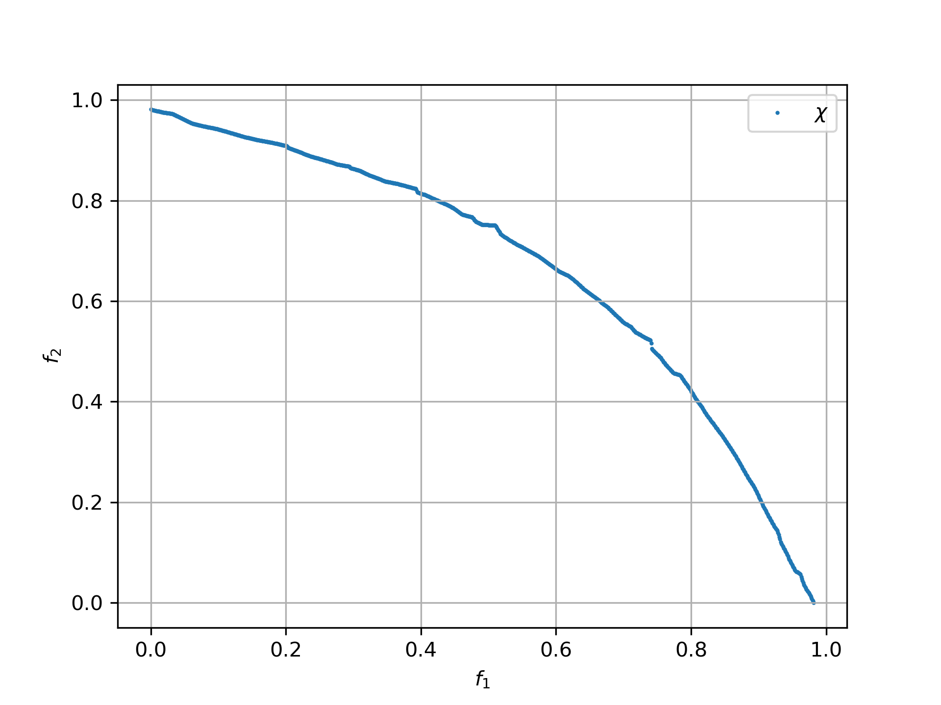
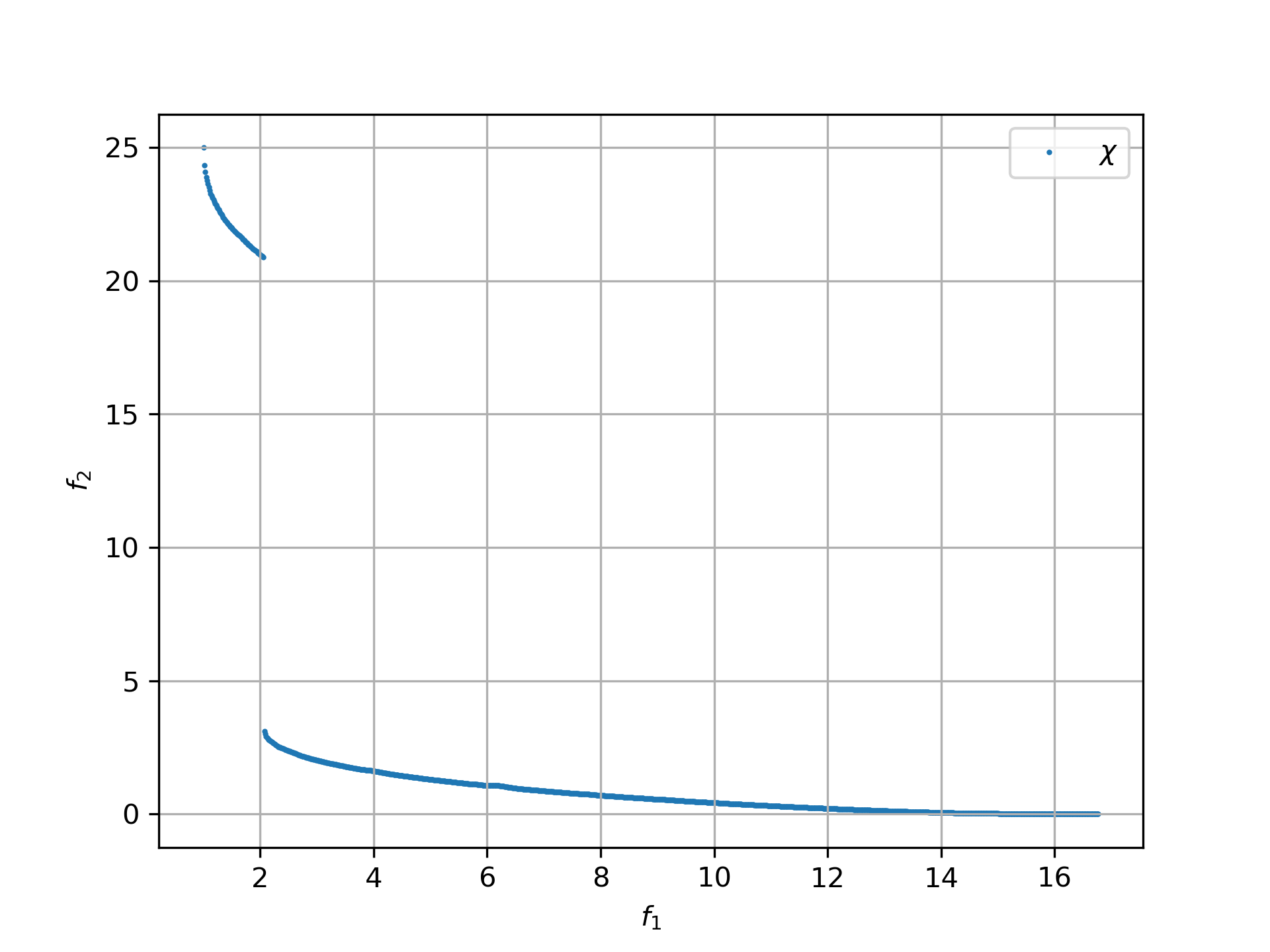
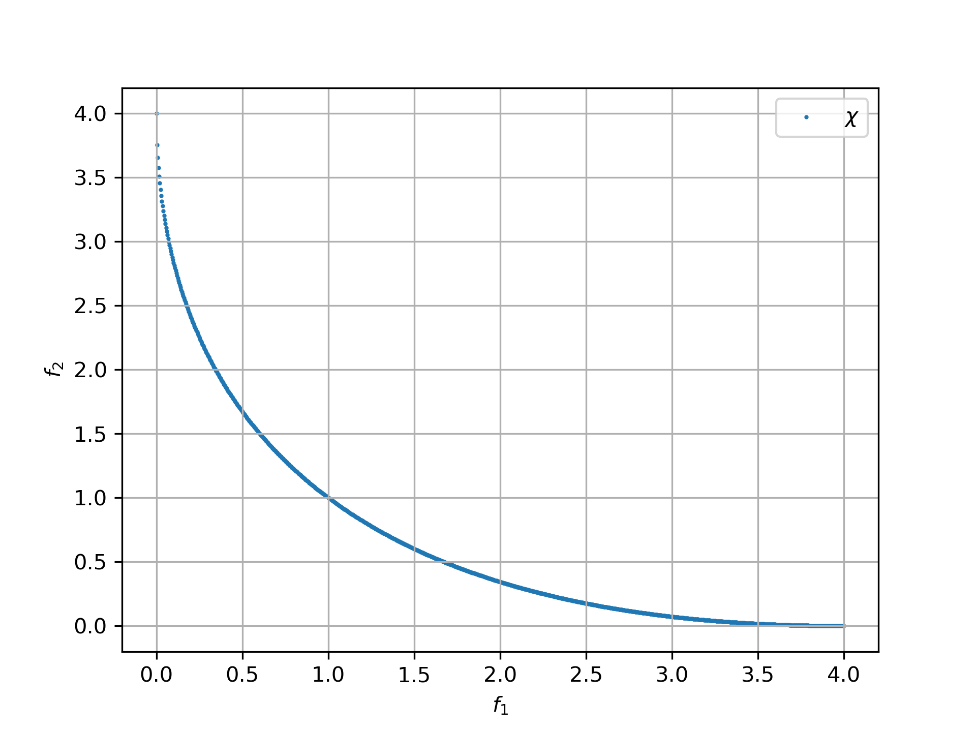
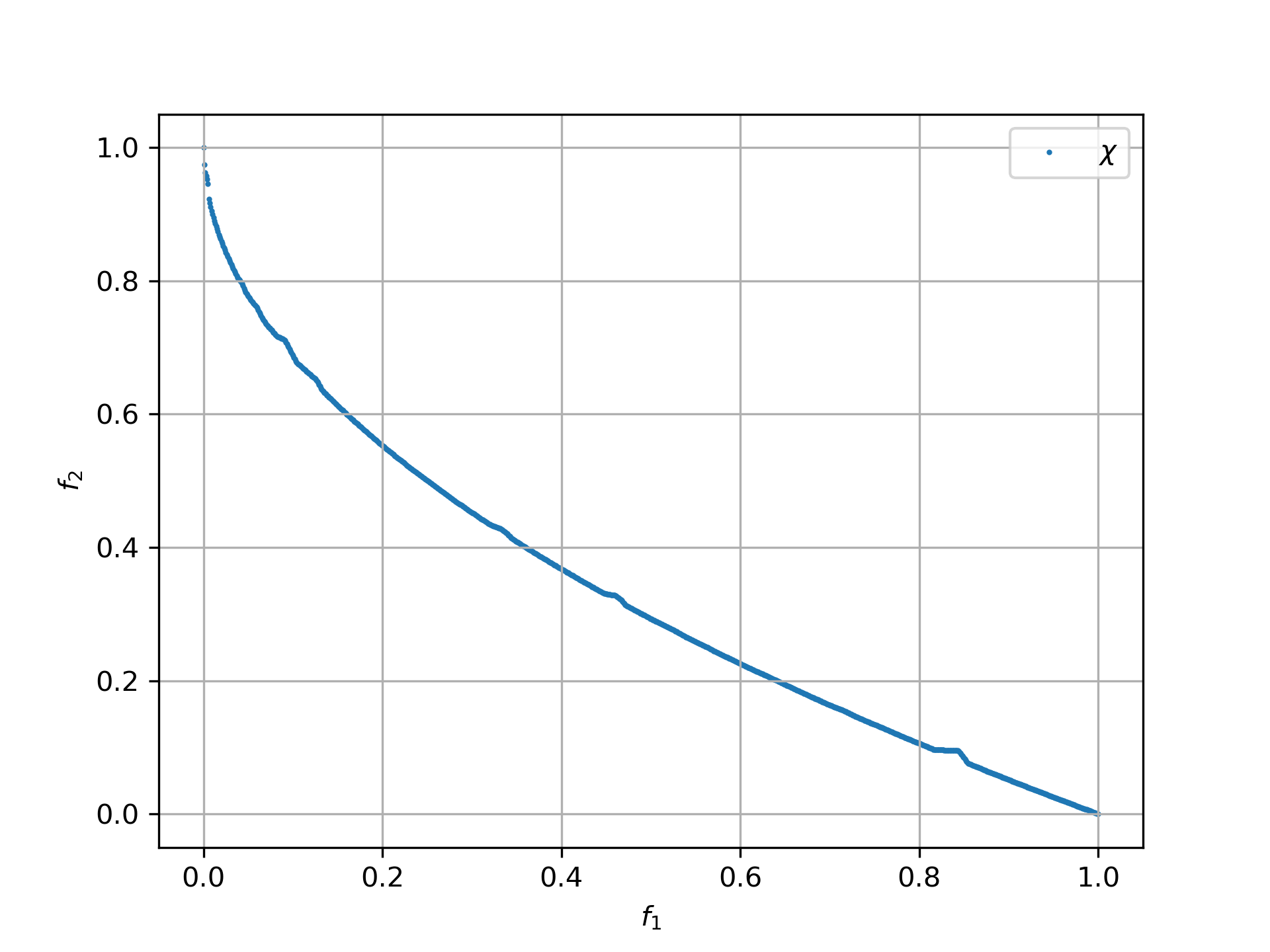
This implementation is single-threaded, but it solves all benchmark problems in under 30 seconds:

Fonseca function, dim = 20, NSGA-II pareto front, NGEN=2000, MU=100:

Poloni function, dim = 20, NSGA-II pareto front, NGEN=2000, MU=100:

Schaffer function, dim = 20, NSGA-II pareto front, NGEN=2000, MU=100:

ZDT1 function, dim = 20, NSGA-II pareto front, NGEN=2000, MU=100:

Given these good benchmark results, it is tempting to expect similar success on Cassini. We know the problem is harder, so we increase the budget to 120000 generations with a population size of 200.

Cassini1 function NSGA-II pareto front, NGEN=120000, MU=200, time = 6587.19 sec:

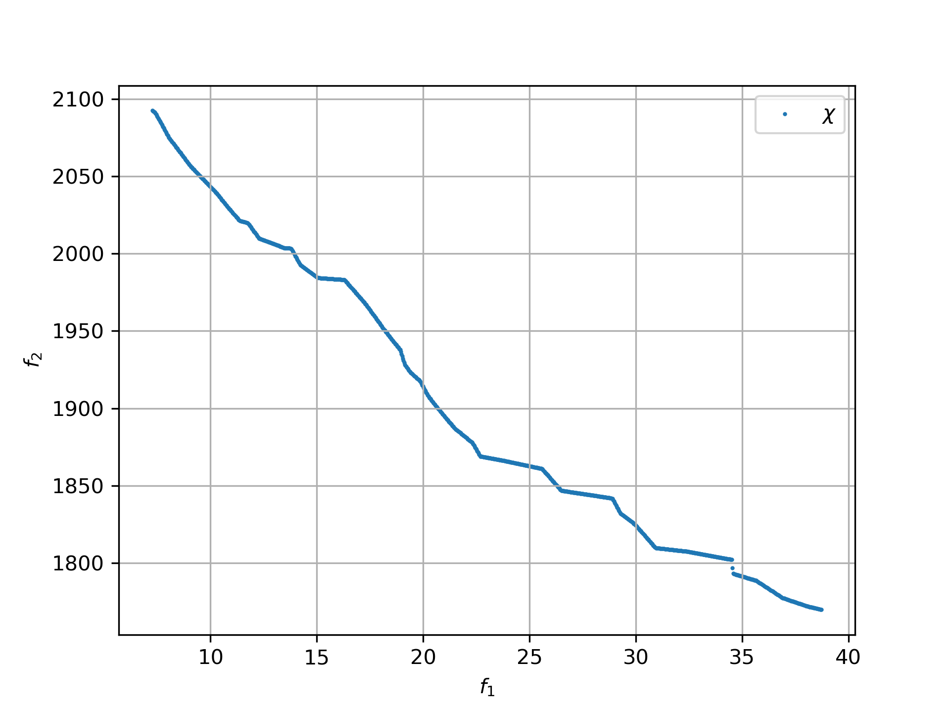
The result is disappointing. Even with 120000 generations and a population size of 200, taking about 6587 seconds, NSGA-II still misses the non-dominated low-dv and high-travel-time solutions.

fcmaes multi objective parallel retry

Our boss is about to leave, so we need a faster approach. The key idea is simple. We take a fast, parallelizable single-objective optimizer, wrap the multi-objective function, and map it to a single objective with a weighted sum.

class mo_wrapper(object):
    """wrapper for multi objective functions applying the weighted sum approach."""

    def __init__(self, fun, weights, y_exp=2):
        self.fun = fun
        self.nobj = len(weights)
        self.weights = weights
        self.y_exp = y_exp

    def eval(self, x):
        y = self.fun(np.array(x))
        return _avg_exp(self.weights*y, self.y_exp)

def _avg_exp(y, y_exp):
    return sum([y[i]**y_exp for i in range(len(y))])**(1.0/y_exp)

We now choose random weights, within predefined bounds, for each optimization retry. Because the retries run in parallel, we can evaluate far more candidate solutions per second.

Why do we need a configurable exponent y_exp? Some Pareto fronts contain very different objective scales. The Poloni function is an example. There we need a low exponent:

Poloni weighted sum, y_exp = 1.0, 2000 evals, 1024 retries, 2.7 sec:

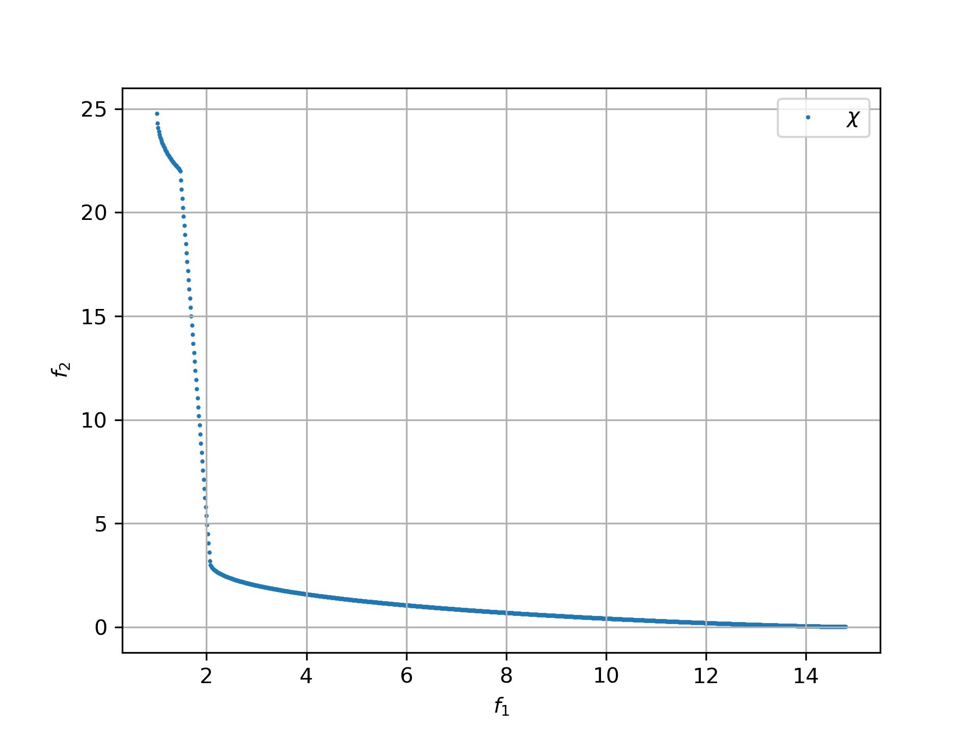
With a higher exponent, we would lose the extreme values on the left. For real-world problems, that is often acceptable because we usually prefer balanced solutions. For the Cassini mission, there may even be hard limits for both travel time and fuel consumption.

For functions like Fonseca, the opposite happens. With low exponents, the Pareto front develops a gap in the middle. That is why we increase the exponent to 3.0:

Fonseca weighted sum, y_exp = 3.0, 2000 evals, 1024 retries, 4.9 sec:

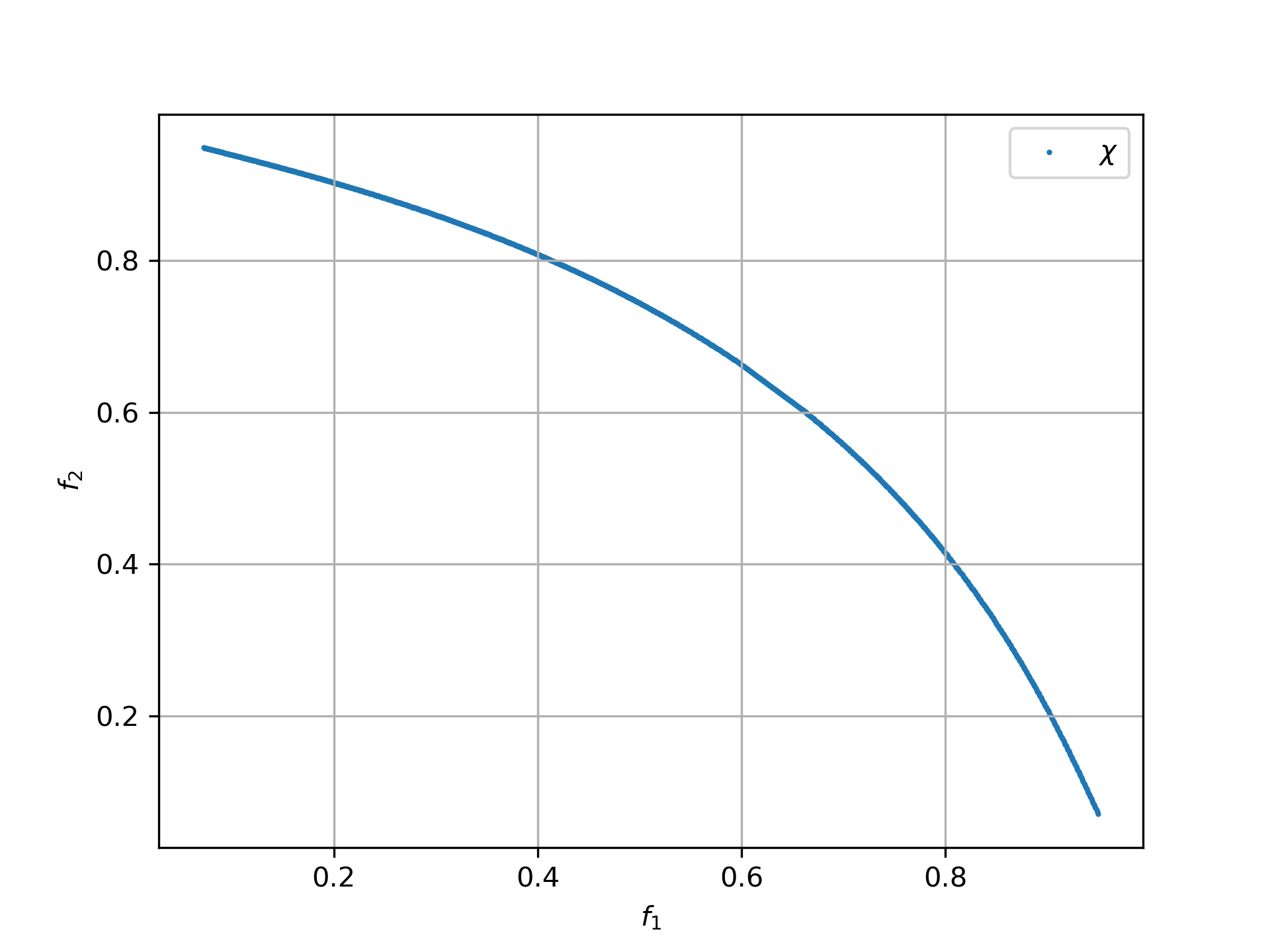
For real-world problems, the default y_exp = 2.0 is usually a good choice.

We configure 1024 retries with a maximum of 50000 evaluations each. Our processor supports 32 parallel threads, so we choose a retry count divisible by 32.

def minimize_plot(name, optimizer, fun, bounds, weight_bounds,
                  value_limits = None, num_retries = 1024,
             exp = 2.0, workers = mp.cpu_count(), logger=logger(), statistic_num = 0):
    time0 = time.perf_counter() # optimization start time
    name += ' ' + optimizer.name
    logger.info('optimize ' + name)
    xs, ys = minimize(fun, bounds,weight_bounds,
             value_exp = exp,
             value_limits = value_limits,
             num_retries = num_retries,
             optimizer = optimizer,
             workers = workers,
             logger=logger, statistic_num = statistic_num)
    retry.plot(ys, 'all_.' + name + '.png', interp=False)
    np.savez_compressed(name, xs=xs, ys=ys)
    xs, front = pareto(xs, ys)
    logger.info(name + ' time ' + str(dtime(time0)))
    retry.plot(front, 'front_.' + name + '.png')

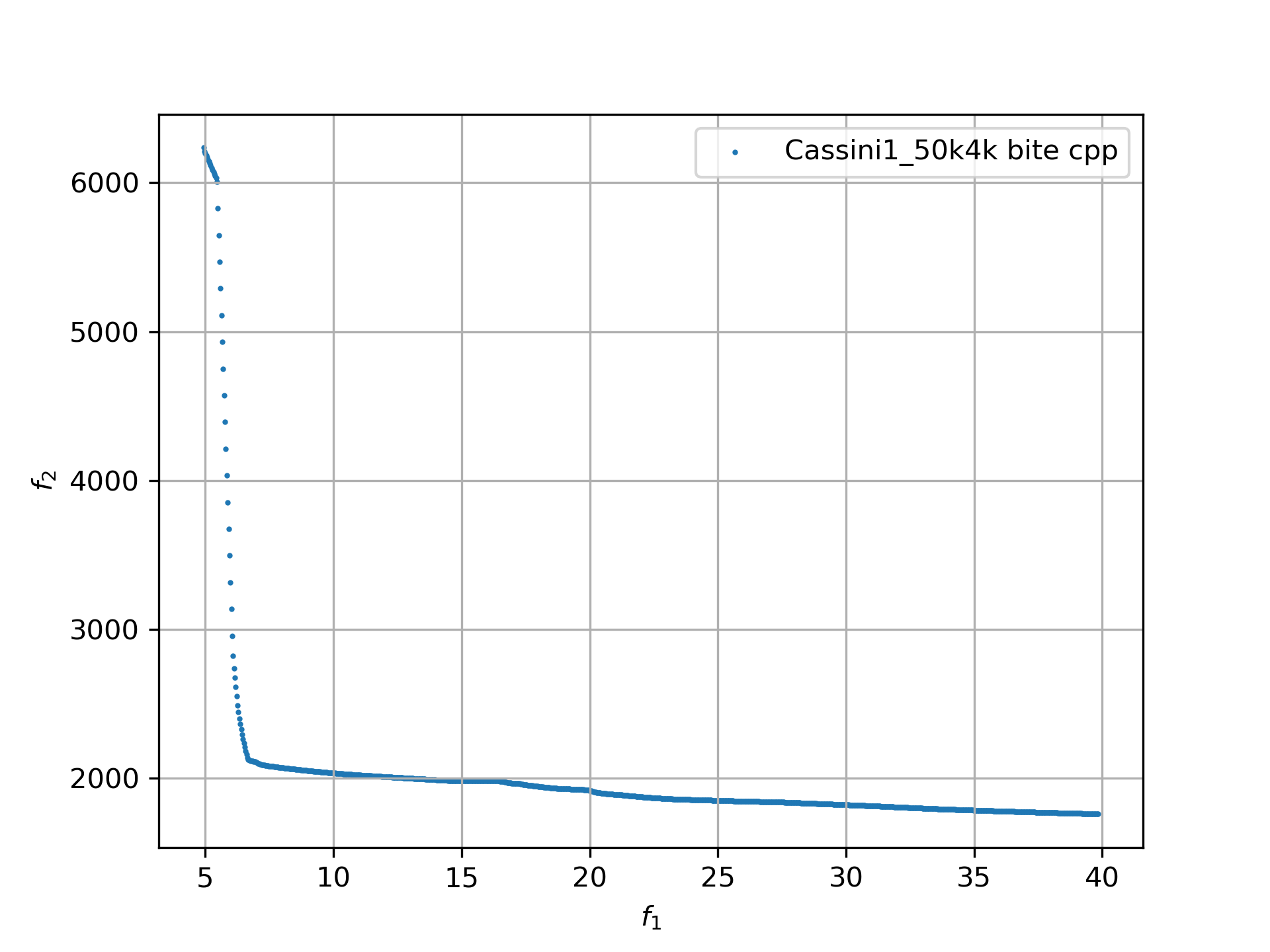
Cassini weighted sum, 1024 retries, max 50000 evals, BiteOpt algorithm, time = 43.62 sec:

Cassini weighted sum, 1024 retries, max 50000 evals, DE-CMA sequence, time = 31.94 sec:

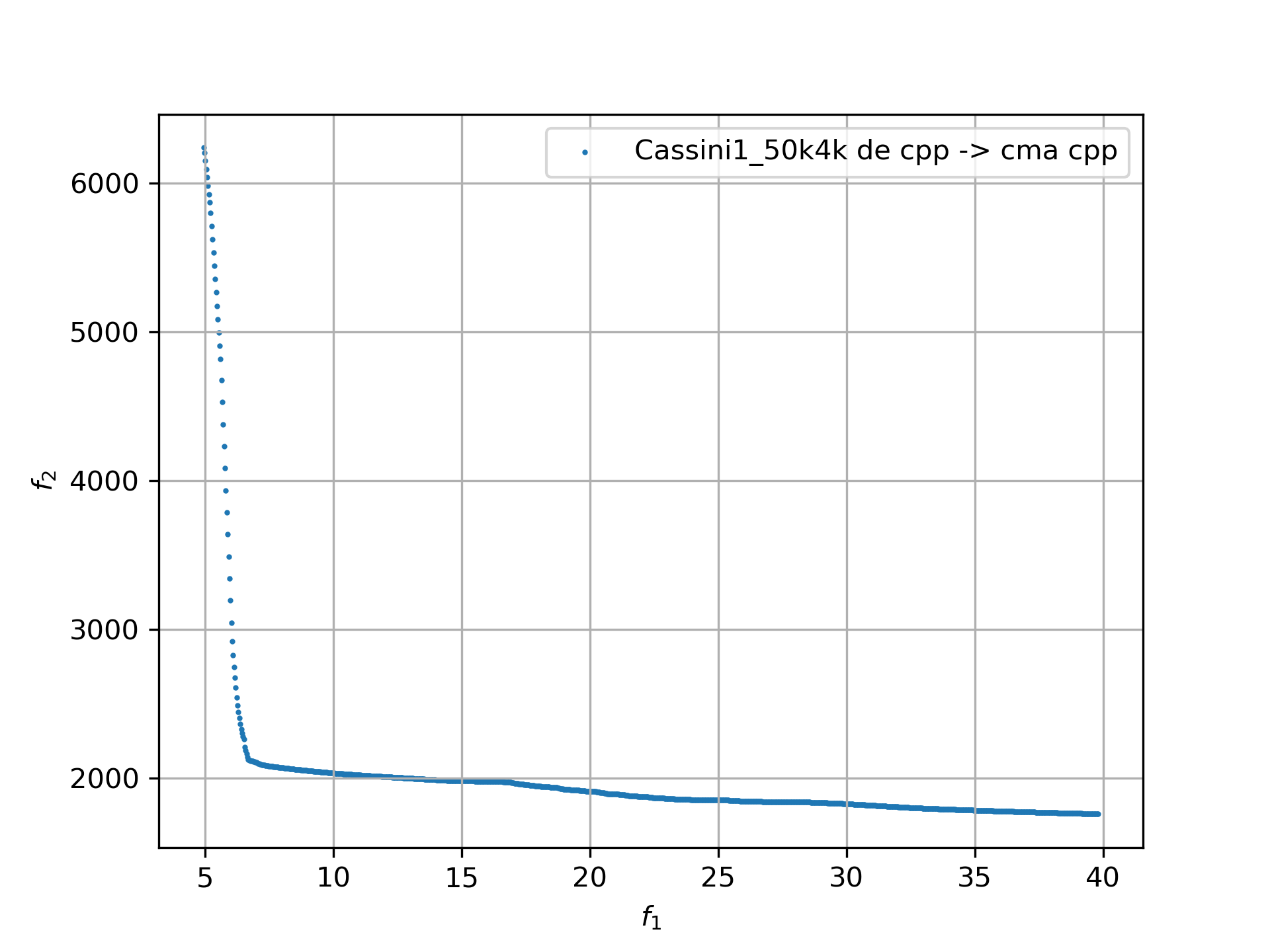
Now the non-dominated low-dv solutions with travel times > 6000 finally appear. Finding this dv optimum is not trivial even in the single-objective formulation. That may explain why NGSA-II fails here.

fcmaes parallel retry outperforms NGSAII by a large margin and also delivers a better result. The main extra requirement is that we extend the function definition with weight_bounds, which defines the range of the randomly generated objective weights. The first objective is in m/s, with an optimum around 4.7 m/s. The second is in days, with an optimum > 1000 days. We therefore define weight_bounds = Bounds([1, 0.01], [100, 1]) to balance the weighted sum. With that, we get a Cassini Pareto front good enough to argue for a maximal mission time of 2100 days.

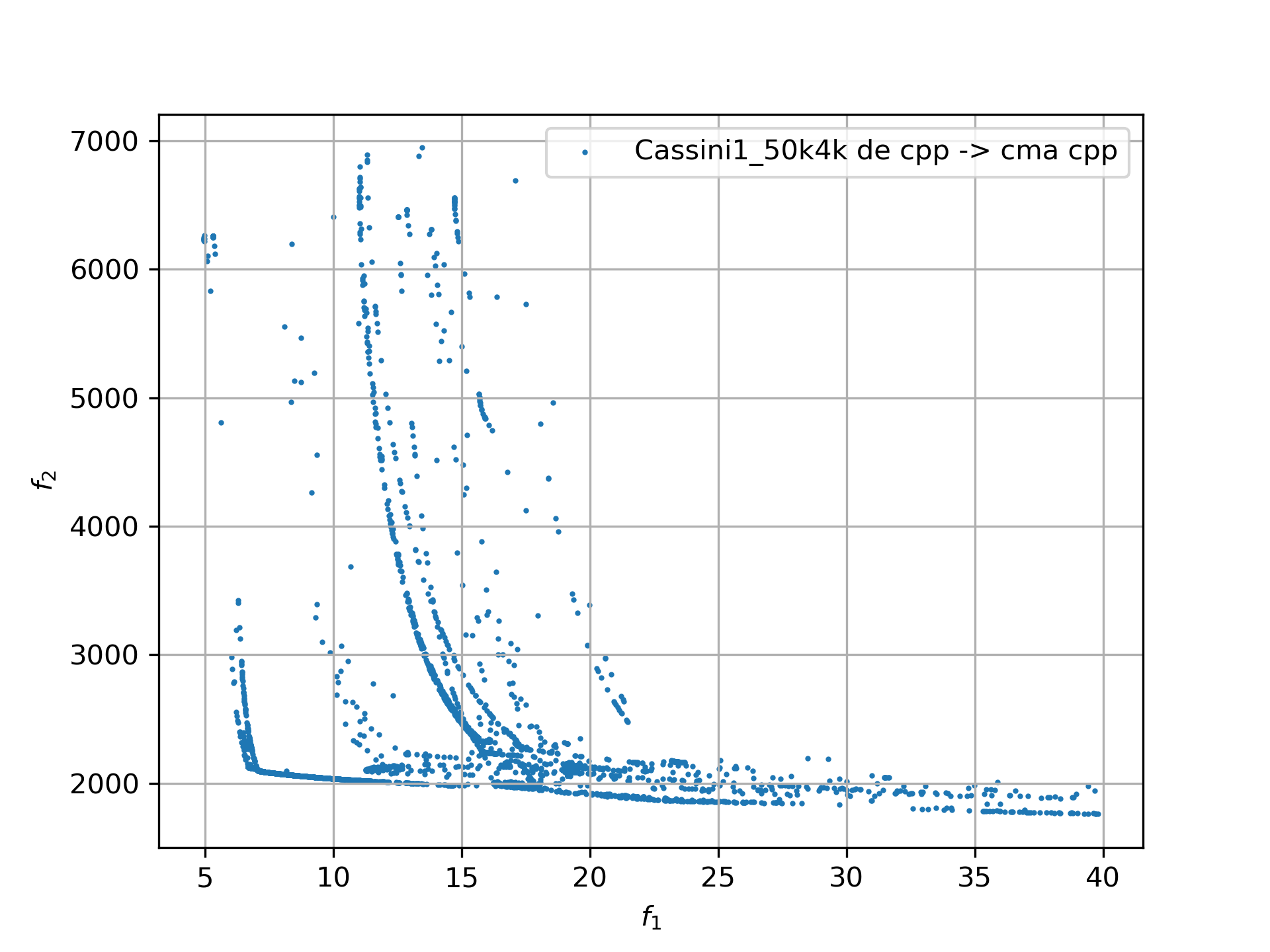
We also save the raw optimization results before applying moretry.pareto, so they can be plotted later if needed:

    with np.load('fname.npz') as data:
        xs = data['xs']
        ys = data['ys']
        moretry.plot(ys, 'fname.png', interp=False)

Cassini weighted sum, 1024 retries, max 50000 evals, DE-CMA sequence, all optimization results:

Constraints

What if the problem must satisfy constraints? One practical option is to convert each constraint into an objective:

Equality: a = b can be converted into objective abs(a-b)
Inequality: a < b can be converted into objective max(0, a-b)

Use high weight-bound values, such as [1000, 1000], to avoid variation in the constraint weights. Sometimes it also helps to add a constant penalty c:

Equality: a = b can be converted into objective abs(a-b) + c if abs(a-b) > 0 else 0
Inequality: a < b can be converted into objective a-b + c if a-b > 0 else 0

What if the problem is crazy hard ?

Now we move to a problem that pushes even state-of-the-art single-objective optimizers close to their limits. Consider the unconstrained variant of ESA’s Tandem problem, another interplanetary trajectory design task with multiple gravity assists. nsgaII_cassini1_mo_20k200_front It took about 3 years until a 1673.88 kg solution was discovered by G. Stracquadanio, A. La Ferla and G. Nicosia at the University of Catania, see https://www.esa.int/gsp/ACT/projects/gtop/tandem_unc . As usual, we import the GTOP problem and modify it so that mission time becomes the second objective:

from fcmaes.astro import Tandem

class tandem_mo:

    def __init__(self, constrained=False):
        self.base = Tandem(5, constrained=constrained)
        self.bounds = self.base.bounds
        self.weight_bounds = Bounds([1, 0], [1, 0]) # ignore 2nd objective
        self.name = self.base.name

    def fun(self, x):
        final_mass = self.base.fun(np.array(x)) # original objective (-kg)
        mission_time = sum(x[4:8]) # mission time (days)
        y = np.empty(2)
        y[0] = final_mass
        y[1] = mission_time
        return y

Let us start with random search:

Tandem unconstrained, 10000 retries 100000 evaluations each:

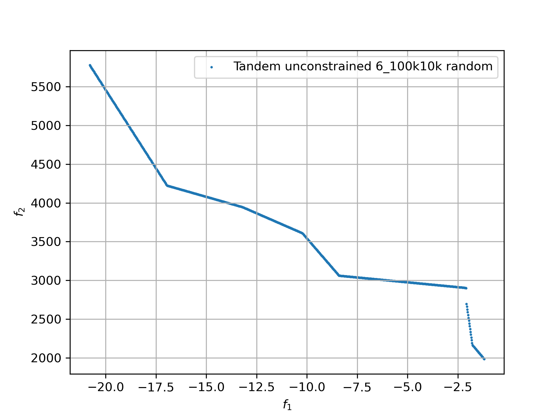
That is a billion evaluations for a maximal mass of 22 kg. The true optimum is 1673.88 kg, so we are still very far away. This is a clear sign that the problem is extremely hard.

NSGA-II

Random sampling gives us no chance here, which is no surprise. So let us try NSGA-II next:

nsgaII_test(tandem_mo(), '_front.png', NGEN=120000, MU=200, value_limits = [0, 10000])

Tandem unconstrained, NSGA-II pareto front, NGEN=120000, MU=200, time = 7245 sec

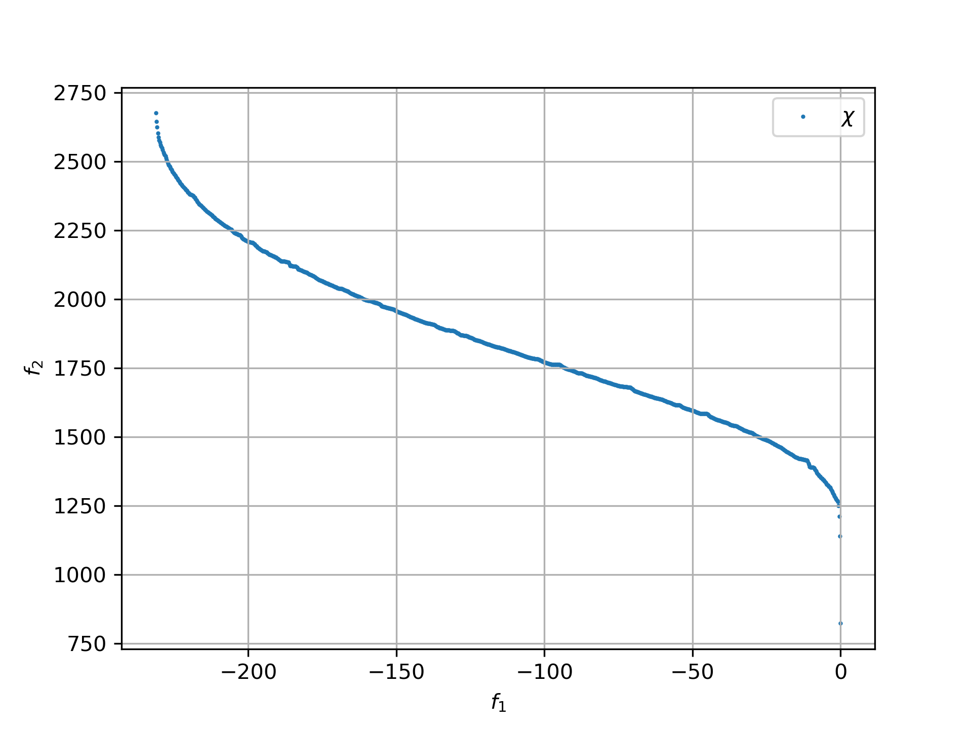
This took over 2 hours. The result looks smooth, but it is still far from the real Pareto front. Below 3000 days of travel time there are hardly any better solutions. Why does NSGA-II avoid longer trajectories? The second objective seems to drag the search away from high-final-mass solutions. With the weighted-sum approach, we can counteract that effect.

fcmaes parallel retry

    minimize_plot(tandem_mo(), de_cma(100000), '100k10k', num_retries=10240, exp=1.0)

Tandem unconstrained, parallel retry de_cma, 100000 evaluations, 4096 retries, time = 556 sec

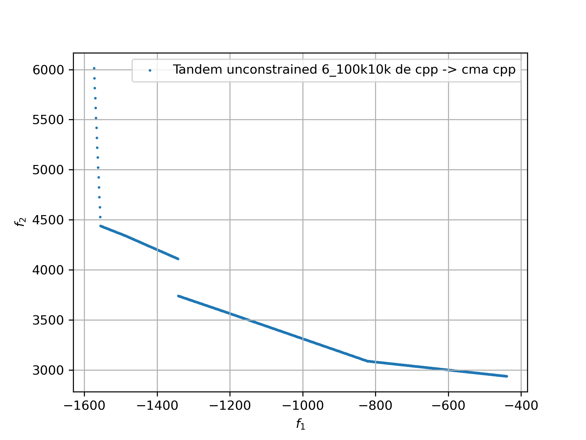
front .Tandem unconstrained 6 de cpp cma cpp

To handle the complexity of the problem, we increase the number of evaluations per retry to 100000. To avoid the drag toward low mission-time solutions, we completely block the second objective with weight_bounds = Bounds([1, 0], [1, 0]) and use exp=1.0, which makes the weighted sum identical to the first objective. That means we could also have used the single-objective Tandem version directly. We do not do that yet, because it enables the next step.

Excercise

Experiment with other weight_bounds and exp settings. You will see that keeping the first objective unchanged is crucial here. Also try other algorithms. Bite_cpp(100000, M=16) is probably the strongest competitor, and on many other problems it can even be better.

Since we optimize only the first objective, we can also try advanced retry. This method adjusts search boundaries using information from previous runs. We pass problem.base.fun, the single-objective Tandem function, to the optimizer. The Pareto front is then computed afterwards using ys = np.array([problem.fun(x) for x in xs]), which applies the multi-objective Tandem function to the optimized solutions.

from fcmaes import advretry

def adv_minimize_plot(name, optimizer, fun, bounds,
                   value_limit = math.inf, num_retries = 1024, logger=logger(), statistic_num = 0):
    time0 = time.perf_counter() # optimization start time
    name += ' ' + optimizer.name
    logger.info('smart optimize ' + name)
    store = advretry.Store(lambda x:fun(x)[0], bounds, capacity=5000, logger=logger,
                           num_retries=num_retries, statistic_num = statistic_num)
    advretry.retry(store, optimizer.minimize, value_limit)
    xs = np.array(store.get_xs())
    ys = np.array([fun(x) for x in xs])
    retry.plot(ys, 'all_smart.' + name + '.png', interp=False)
    np.savez_compressed(name , xs=xs, ys=ys)
    xs, front = pareto(xs, ys)
    logger.info(name+ ' time ' + str(dtime(time0)))
    retry.plot(front, 'front_smart.' + name + '.png')

adv_minimize_plot(tandem_mo(), de_cma(1000), '_' + str(i) + '_smart', value_limit = -500, num_retries = 100000)

Tandem unconstrained, parallel smart retry de_cma, 100000 retries between 1000 and 50000 evaluations, time = 3360 sec

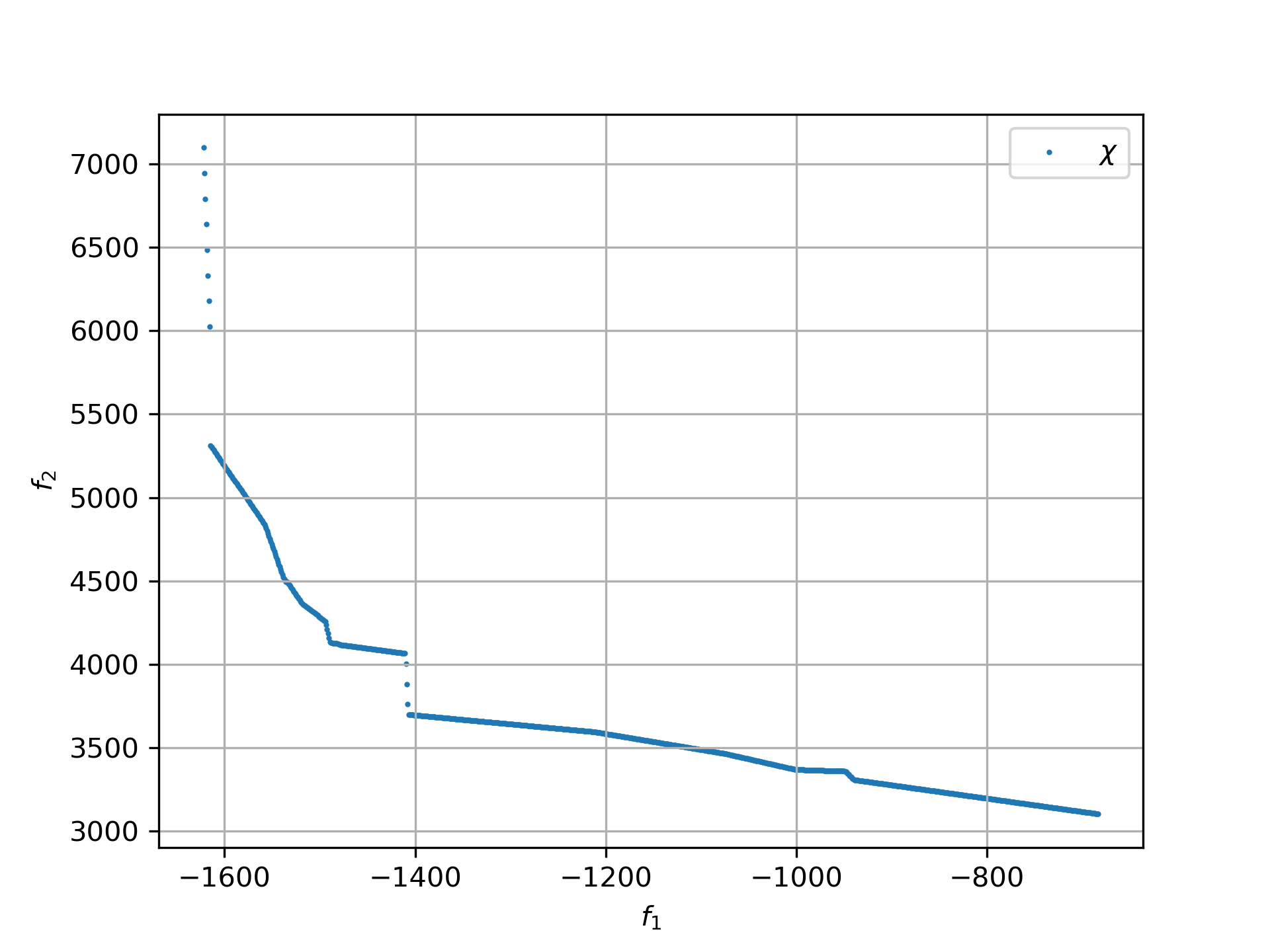
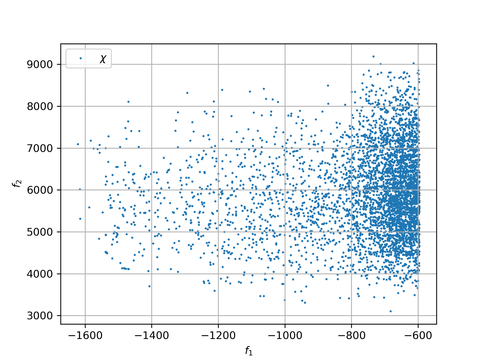
If we inspect all generated solutions, we see that the smart parallel retry algorithm found three solutions above 1600 kg.

Joined forces

A single run may not be enough to approximate the Pareto front well. That is why we saved the optimization results using np.savez. We can now collect those files and build a final result:

def plot_all(folder, fname):
    files = glob.glob(folder + '/*.npz', recursive=True)
    xs = []
    ys = []
    for file in files:
        with np.load(file) as data:
            xs += list(data['xs'])
            ys += list(data['ys'])
    xs = np.array(xs); ys = np.array(ys)
    xs, front = moretry.pareto(xs, ys)
    moretry.plot(ys, fname + '_all.png', interp=False)
    moretry.plot(front, fname + '_front.png')

What if the problem is not solvable even as single objective problem ?

Then we need a surrogate model. _solar_orbiter_udp_1dsm models the Solar Orbiter mission as a sequence of gravity assists with a single deep-space maneuver (1DSM) between planets. Assume we use the planet sequence

seq=[earth, venus, venus, earth, venus, venus, venus, venus, venus, venus]

as in the original mission. The 1DSM Solar Orbiter model is very general and allows solutions that were not considered by the original planning team at ESOC. Unfortunately, solving it directly would require future optimization algorithms and an enormous amount of computing power. So our first goal is more modest. We want to establish that the model is correct by reproducing several good solutions that we already know from a much simpler model, which we fortunately already have here: solo_mgrar_udp.py. Using this surrogate model, we can compute solutions that can later be converted into solutions of the 1DSM model. That conversion includes a local optimization with the 1DSM model for each surrogate solution because of accuracy issues. Here we listed solutions for both Solar Orbiter models. There is no realistic chance to apply existing multi-objective algorithms like NSGA-II to either the 1DSM model or the surrogate model.

Solar Orbiter has not just two, but several competing primary objectives:

Minimal delta velocity / fuel consumption
Minimal overall travel time
Maximal inclination relative to the sun equator - we want to investigate the poles of the sun.
Minimal - but limited - perhelion. We want to come close but avoid burning our equipment.

For this example, we choose the following two objectives:

First objective: maximal inclination in deg.
Second objective: minimal travel time in days.

Solar Orbiter 1DSM model, all combined optimization results:

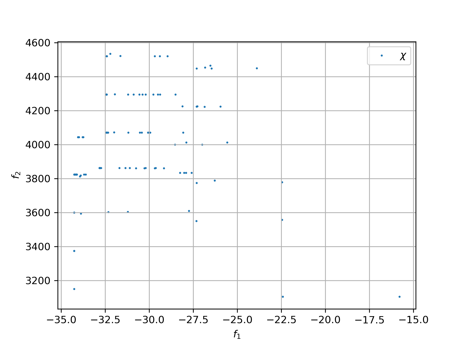
Solar Orbiter 1DSM model, pareto front of all combined optimization results:

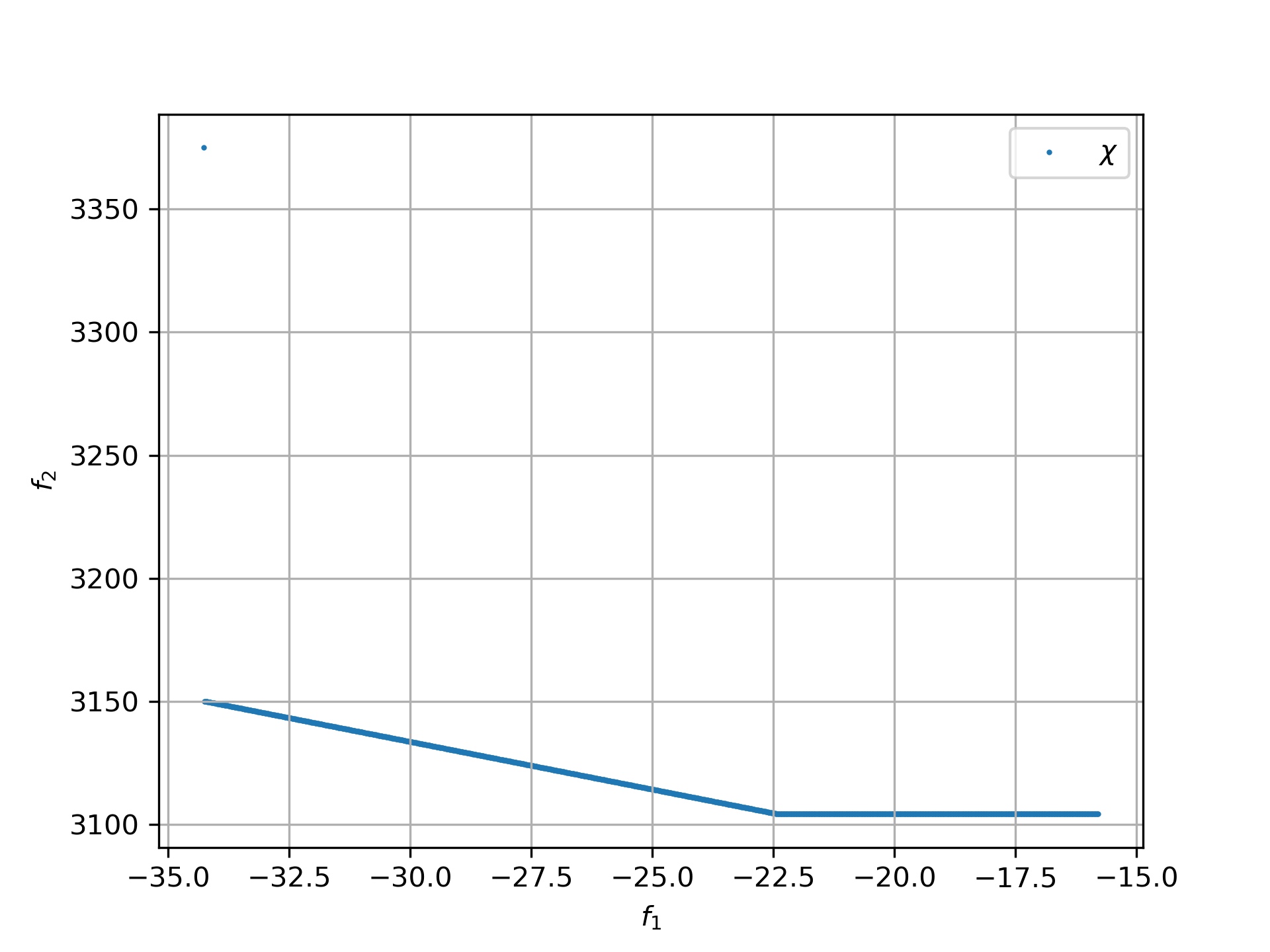
Here the Pareto front is not the most useful output. Instead, we keep all good solutions and select one later using secondary objectives such as:

Do we cross a comet halo? The real Solar Orbiter mission does, although this was not part of the planning.
Start velocity from earth
Downlink capability - how fast can data be transferred during the mission

See SOL-ESC-RP-05500 for a detailed description of the mission goals.