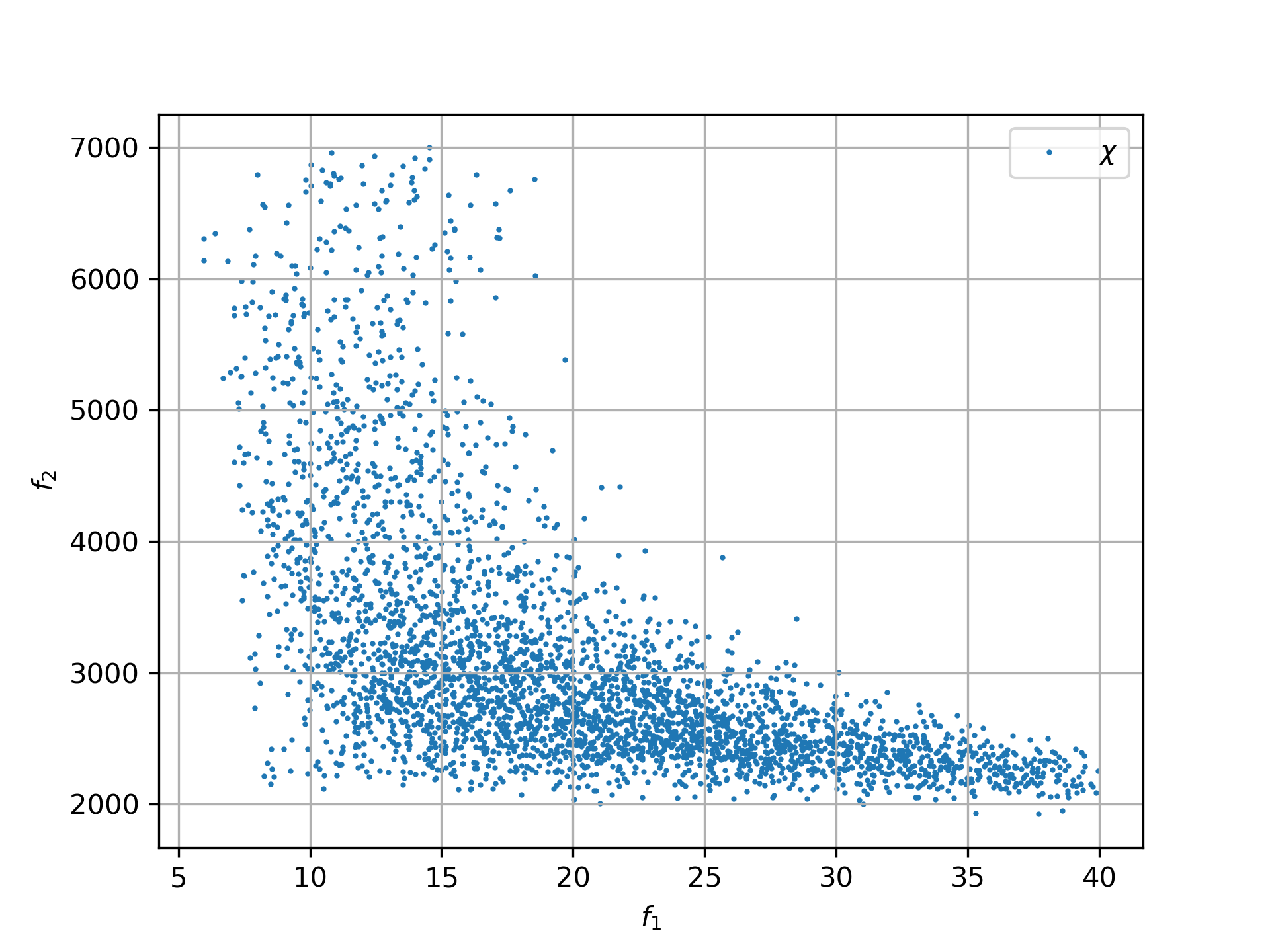
fcmaes - a Python 3 gradient-free optimization library

Multi-objective optimization with MODE

Explains when to use which multi-objective optimization method for which kind of real-world optimization problem.
Discusses a new fcmaes-MODE multi-objective algorithm with constraint support. It comes with two variants:
- NSGA-II population update
- Differential Evolution population update

Motivation

The initial development of fcmaes was driven by applications in space flight mission design. Later, work on other real-world optimization problems added new meta-algorithms for mixed-integer problems, constraints, and multi-objective optimization. Multi-objective methods help us understand the tradeoffs between competing objectives.

When to apply which multi-objective algorithm using Python

If the problem is not trivial, use parallelization. That usually means either using cloud resources or investing in a modern many-core CPU. It also means choosing tools carefully:

If you use an open-source solution, avoid non-Unix operating systems like Windows, or use the Linux subsystem for Windows WSL, because Python multiprocessing has issues on Windows.
If you plan to use pymoo, check first how well its parallelization mechanisms scale. Its overhead is huge for objective functions that are fast to evaluate.
If you plan to use some other open-source optimizer, check whether it supports parallelism on your OS at all, and how well it scales for your problem.

Either implement the objective function in C++ and add a Python interface, for instance using ctypes, or use numba for the time-critical parts if you stay in Python.

Many real-world problems can still be implemented surprisingly efficiently this way, even in Python.

It also helps to optimize a simplified model first, then transfer good results back to the more accurate but harder-to-evaluate model. In space mission design, for example, this can mean using an impulse-based approximation during optimization even if the final system uses continuous thrust.

If you decide to use fcmaes, there are several options:

moretry.minimize

A meta-algorithm that applies a single-objective optimizer through the weighted-sum approach. It runs parallel optimizations with random weights for the objectives to produce a Pareto front. The weight distribution is configurable. Use it only if

The objective function is fast to evaluate, since it needs many evaluations.
There are not more than two objectives.
One objective is strongly connected to one or more decision variables. For instance, the ToF (time of flight) in a space mission when start time is one of the variables. In this case, MO algorithms tend to overemphasize this variable. Using moretry, we can force the focus toward the other objective through the weight distribution.
Only the very best single-objective algorithms have a chance to optimize one of the objectives. An example is delta velocity (fuel consumption) for a multi-planet gravity-assist mission.

mode.minimize

A new fcmaes multi-objective algorithm implemented in Python and equivalent to modecpp.minimize. Use it only if modecpp.minimize has issues:

missing shared library for your OS
problems with parallel fitness function evaluation in your environment

modecpp.minimize

A new fcmaes multi-objective algorithm implemented in C++. Use it if

Your objective function is expensive. In this case, use parallel fitness function evaluation.
Your problem has constraints. With moretry, you need either the weighted-sum or the Chebycheff method. modecpp supports constraints directly.
No objective is directly connected to a decision variable.
There are more than two objectives.

modecpp.retry

The same optimization algorithm as modecpp.minimize and mode.minimize, implemented in C++. It does not use parallel function evaluation. Instead, it performs multiple optimization runs in parallel and joins the results into a single Pareto front. Use it if

Your objective function is fast to evaluate, or you have plenty of time for the optimization.
Any of the other criteria for modecpp.minimize apply.

Scaling, meaning the increase in function evaluations per second per CPU core, is much better with modecpp.retry. Prefer it when the cost of objective function evaluation does not prevent its use.

mode.retry

Doesn’t exist. Use modecpp.retry instead. Or use mode.minimize / modecpp.minimize if your objective function is expensive.

nsga_update

All fcmaes MODE variants have the nsga_update parameter. It determines the population update mechanism: either NSGA-II or DE (Differential Evolution). Try nsga_update=True first, since it tends to produce reasonable results faster. Then try nsga_update=False to see whether results improve in longer runs.

population size

Population size usually needs to be larger than for single-objective algorithms. Use popsize=64 or bigger. modecpp.minimize usually needs a larger population size than modecpp.retry. The same holds for nsga_update=True compared to nsga_update=False. The right value depends on the number of decision variables and the complexity of the problem. Do not exceed popsize=200 in the first experiment. Increase later if necessary.

mixed integer

All fcmaes MODE variants support the ints parameter, but only if nsga_update=False (DE population update) is configured. If you have integer decision variables, use ints to mark them for the algorithm where applicable. The same holds for the single-objective Differential Evolution variants (de.minimize and decpp.minimize).

If you have discrete float input values, use an int-to-float conversion table inside the objective function and denote the variables using the ints parameter.

If you have a permutation as input, do not use ints. Instead, declare the variables as box-constrained floats in the [0,1] interval and use numpy.argsort inside the objective function to produce an integer permutation.

MO-DE a new multiobjective optimization algorithm supporting constraints

In Multi-Objective and gbea TopTrumps Benchmark, we showed that parallel retry with the weighted-sum approach can make sense when combined with strong single-objective optimizers like BiteOpt or fcmaes-DE. Random weights can cover the Pareto front in parallel. For very expensive simulation-based fitness functions, such as TopTrumps, a single run with parallel function evaluation can be a better choice.

For this reason, we adapted the single-objective Python Differential Evolution implementation de.py to multi-objective problems: mode.py. We also added a C++/Eigen-based implementation: modeoptimizer.cpp.

Two ideas from NSGA-II are crucial for MO optimizer performance: fast non-dominated sorting and crowding distance. Both are adapted here. Since DE uses sorting instead of tournament selection, the implementation uses sorting-based variants of these concepts.

For some problems, NSGA-II converged better on parts of the Pareto front. Because of that, we added a configuration parameter that switches the population update mechanism from DE to the NSGA-II update. The NSGA-II update code is derived from GLOBAL.py, which provides an efficient Python implementation.

This gives mode.py some useful features:

It lets you compare DE and NSGA-II population update mechanisms while keeping everything else identical.
It supports parallel execution of the fitness function.
If the NSGA-II population update is chosen, convergence and crowdedness are similar to other NSGA-II implementations.

This suggests that the population update mechanism, not tournament selection, is the crucial part of NSGA-II.

For cheap but difficult fitness functions, such as those derived from ESA’s GTOP space flight trajectory benchmarks, we recommend parallel retry with random weights using moretry.py. mode.py is intended for very expensive fitness functions when your time budget is limited. That is also why no C++ variant of mode.py is implemented yet. For expensive fitness functions, algorithm overhead is relatively low.

It can also make sense to run both variants, DE and NSGA-II population update, with half the time budget each. If you have two machines or processing nodes, run them in parallel. Their weaknesses may cancel each other out.

Comparison to GDE3

GDE3 describes another multi-objective DE algorithm. It is implemented in GDE3.java. JMetal also supports parallel function evaluation and implements NSGAII, but a Java framework is less convenient in a Python environment.

Differences to GDE3 are:

GDE3 uses the DE/rand/1/bin strategy, while mode.py uses the Pareto front to generate offspring. This is similar to the DE/best/1/bin strategy in the single-objective variant.
GDE3 directly compares a new decision vector with its ancestor and decides which one survives based on dominance and crowding value. mode.py sorts the whole population using Pareto hierarchy and crowdedness, and only the best survive. Constraint support in mode.py is implemented as follows: We compute, and prioritize, the Pareto hierarchy for feasible decision vectors, then the constraint Pareto hierarchy for the infeasible ones. The crowdedness or diversity value matters only at the hierarchy level that lies on the population-size border, since diversity has the lowest priority in the survival decision.
GDE3 uses a variable population size because of the direct-comparison approach. If neither of two decision vectors dominates the other, both stay in the population. mode.py’s sorting mechanism avoids this. That can be an advantage for parallel fitness function evaluation. If population size is fixed and is a multiple of the maximum number of parallel CPU threads, CPU utilization is better.
GDE3 implements only one population update strategy. If you optionally switch it to NSGA-II as mode.py does, the resulting algorithm can no longer be called "Differential Evolution".

Another NSGA-II implementation with parallel function evaluation is available in Pygmo/Pagmo, but parallel function evaluation is difficult there when the fitness function is implemented in Python.

Crowdedness

Multi-objective optimizers have to satisfy two criteria:

Convergence: How far is the computed Pareto front "above" the real Pareto front?
Crowdedness/diversity: How evenly are the computed results distributed along the Pareto front?

There is also a third criterion that is often missing:

Coverage: Is the whole Pareto front covered?

Coverage is not the same as crowdedness. The following example shows the difference.

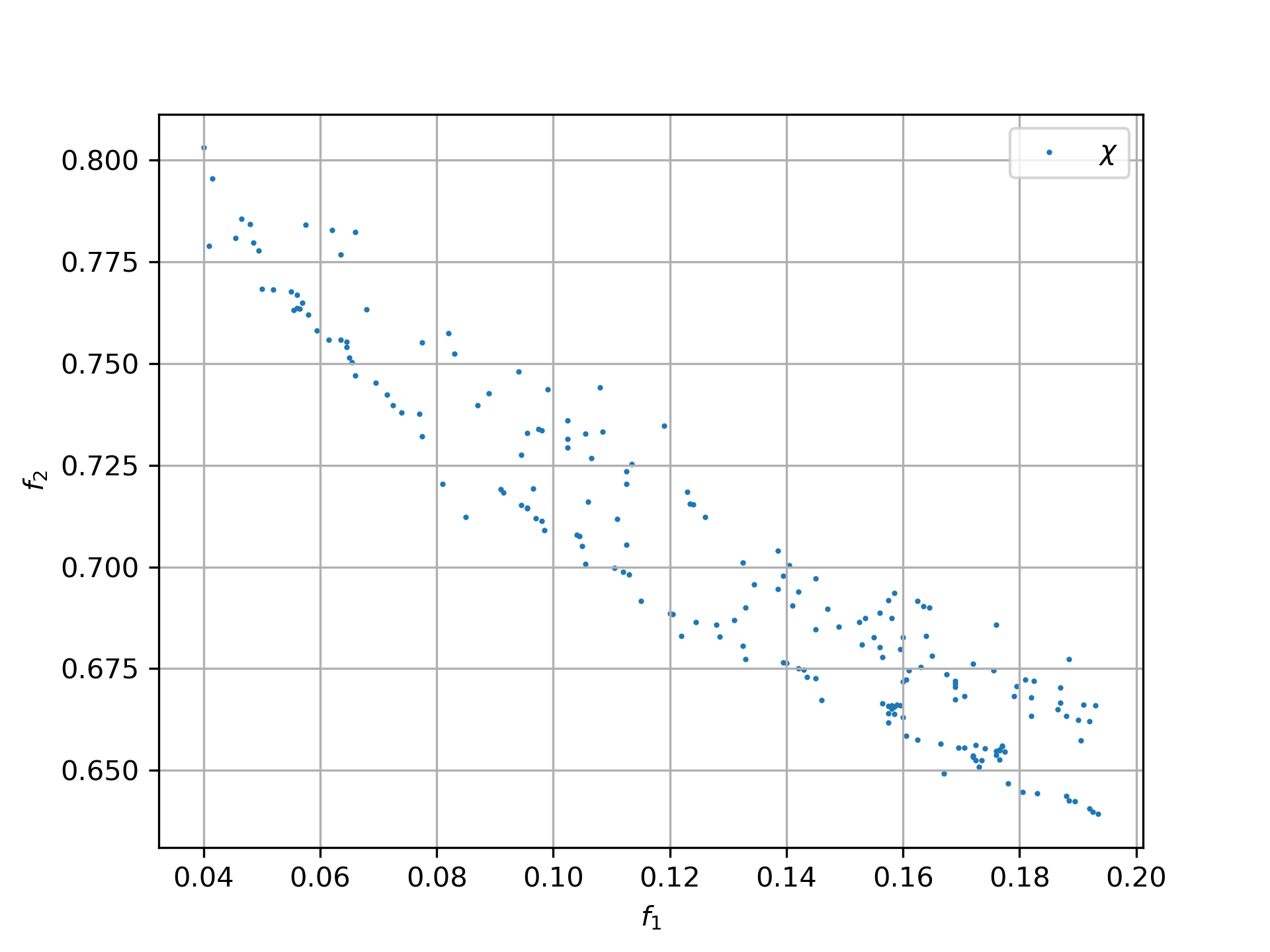
Both results represent optimization runs for the second multi-objective TopTrump benchmark, variant 5, dimension = 128. See Single- and multi-objective game-benchmark for evolutionary algorithms or GBEA.

Application of (mode.py) with popsize = 200, 500k evaluations, NSGA-II population update:

all rw top trumps biobj f2i5d128 mode 200 500k ngsa up

Application of DE (moretry.py), popsize=31 using 512 weighted sum parallel retries, 8k evaluations each:

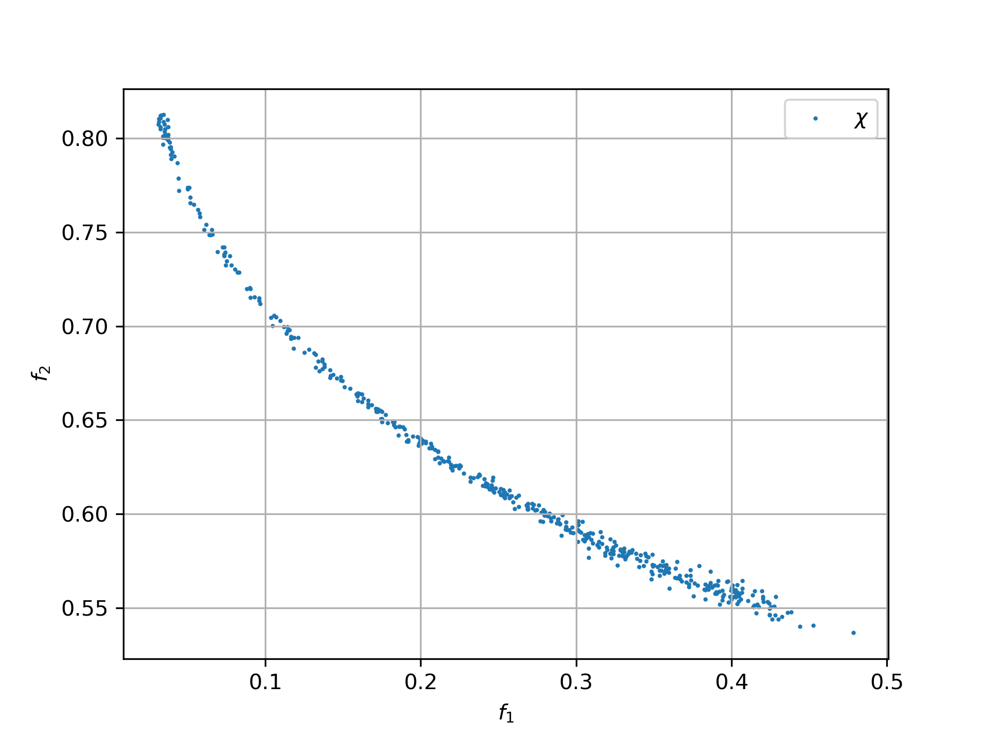
all rw top trumps biobj f2i5d128r2000 8k512 de cpp

Both algorithms use parallelization, but the second test uses a much higher budget. In both cases, crowdedness and convergence are not the main problem. In the first experiment, a large part of the Pareto front is simply missing.

This issue is highly relevant in practice, but it seems underrepresented in the literature. It mostly appears on hard real-world problems. Fortunately, real-world MO problems such as TopTrumps are becoming more common in optimization research.

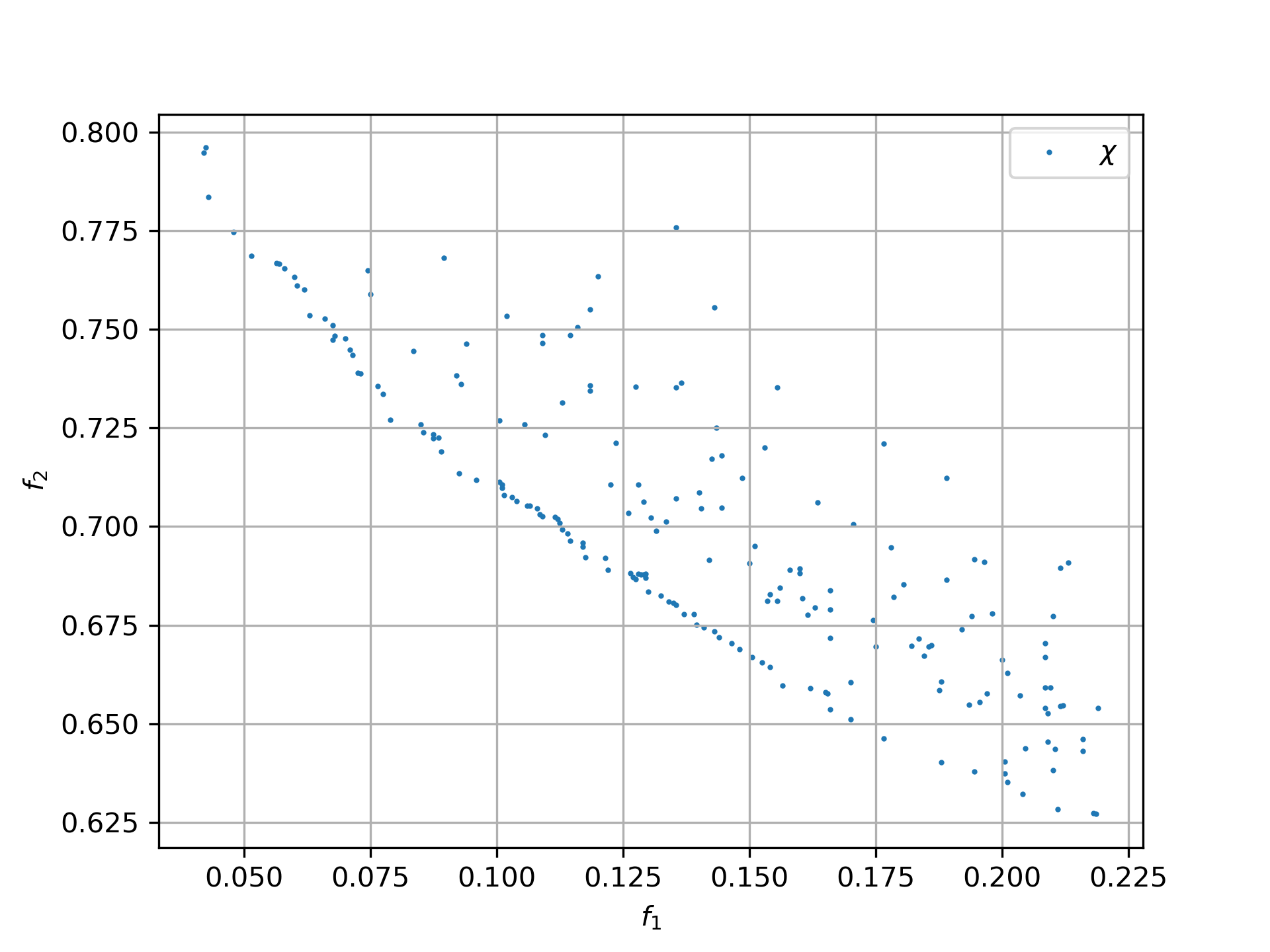
Because the issue is underrepresented, the method that addresses it is often underrated as well: the weighted-sum approach with random weights applied to parallel retries, as implemented in moretry.py. Keep this in mind when using mode.py with parallel fitness function evaluation instead. NSGA-II and DE may miss parts of the Pareto front. To be safe, try moretry.py with a limited budget. You may lose crowdedness and convergence, but gain coverage. At least you will see the issue and can rethink your budget decision. The DE population update is affected as well, although a bit less in this example:

Application of (mode.py) with popsize = 200, 500k evaluations, DE population update:

all rw top trumps biobj f2i5d128 mode 200 500k de up

But other problems show the opposite behavior. One example is the bi-objective variant of ESA’s Cassini1 space mission design benchmark, using mission time as the second objective.

Application of (mode.py) with popsize = 200, 1000k evaluations, NSGA-II population update:

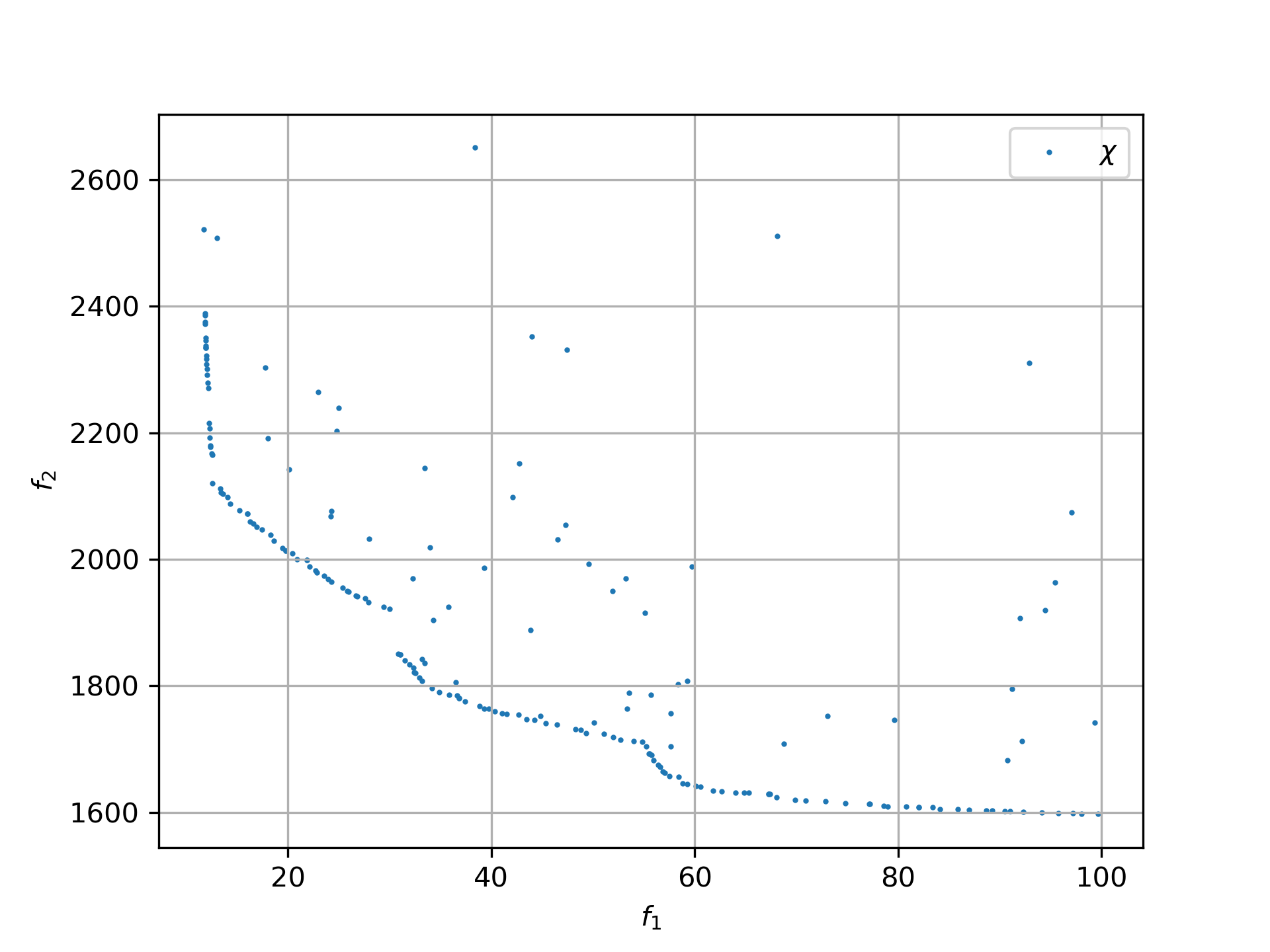
Application of (mode.py) with popsize = 200, 1000k evaluations, DE population update:

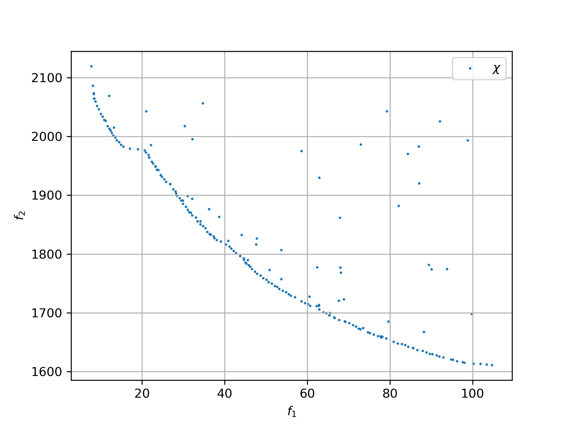
Here the left side looks good, but there are convergence issues on the right side. Let’s try a second run:

Application of (mode.py) with popsize = 200, 1000k evaluations, DE population update, 2nd try:

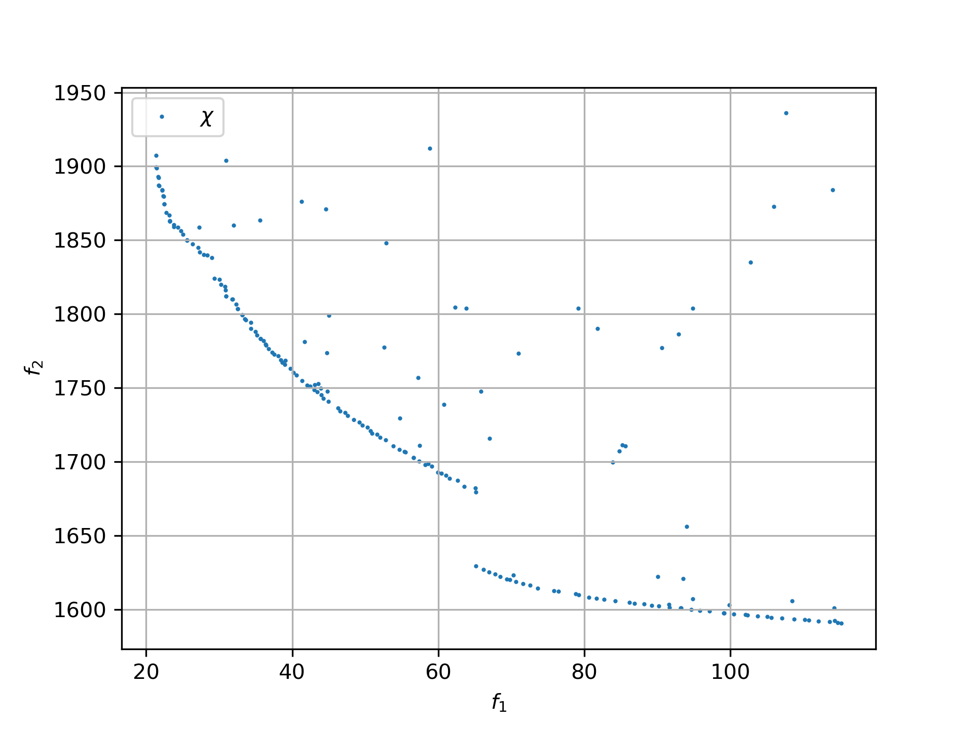
Now part of the left side is missing. We may be able to use this diversity across retries to our advantage by merging results into a single set. We did not observe this kind of diversity for the NSGA-II update, at least not with population size 200. So if you plan only one run, the NSGA-II update may be the better choice.

All of these results still miss a small part of the Pareto front on the left. The low delta-velocity (first objective) solutions using more than 6000 days (second objective) are missing, as shown here:

Application of a DE-CMA sequence using (moretry.py), popsize=31 using 4k weighted sum parallel retries, 50k evaluations each:

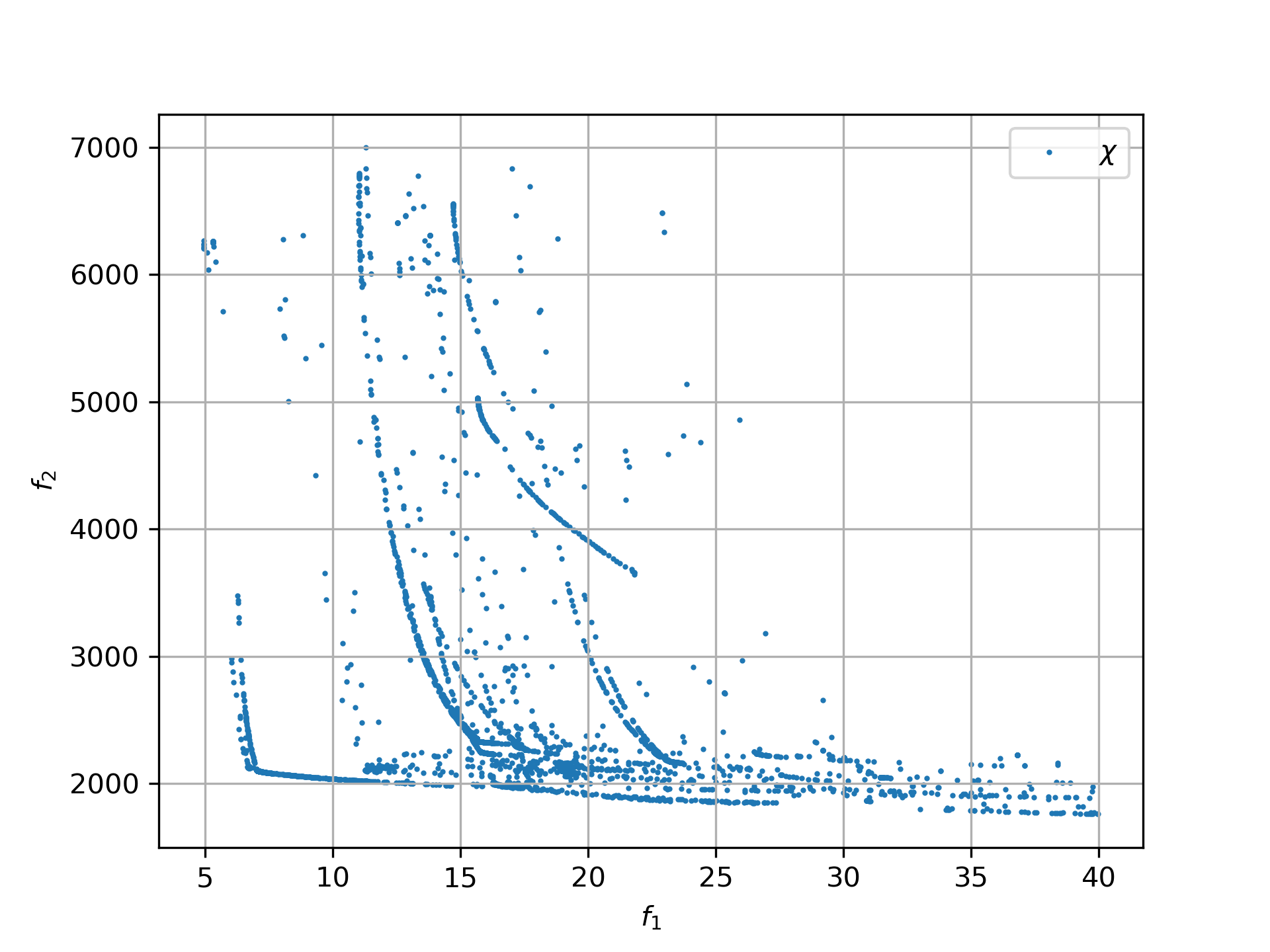
The right side was cut on purpose here to focus on the more interesting low-delta-velocity part of the Pareto front. These weighted-sum experiments can also reveal useful properties of the single-objective algorithms being used. Although the Pareto front is quite similar, the equivalent picture for the BiteOpt algorithm looks very different:

Application of the BiteOpt algorithm using (moretry.py), using 4k weighted sum parallel retries, 50k evaluations each: