fcmaes - a Python 3 gradient-free optimization library

Optimization of functions solving differential equations

This tutorial:

Applies continuous optimization to problems involving the solution of ODEs.
Discusses different ways to solve ODEs in Python. In some cases it is better to define them in C++ and call that code from Python.
Shows how to apply parallel optimization.

Note that recently there are new alternatives you should also consider:

heyoka which helps when there are high accuracy requirements,
desolver.

Rabbits and Foxes

During World War I, complete fishery closure caused an increase in predatory fish and a decrease in prey fish. This counter-intuitive observation led Alfred Lotka and Vito Volterra to independently develop mathematical models of predator-prey population dynamics in the 1920s.

This idea is expressed as a set of differential equations. The scipy tutorial lotka-volterra-tutorial covers it well. It uses foxes as predators and rabbits as prey. Here is a visualization of the solution:

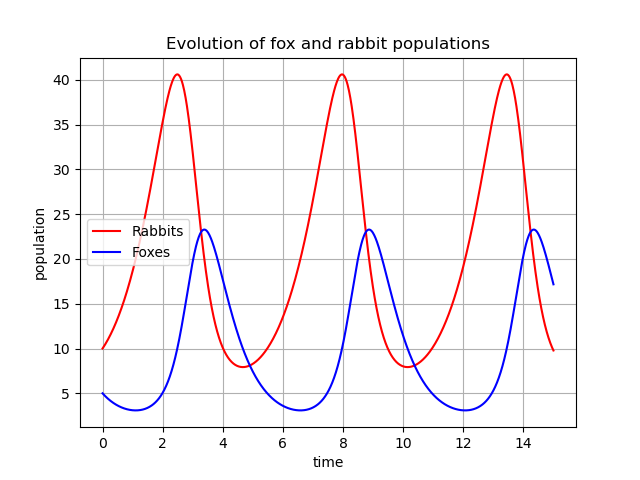
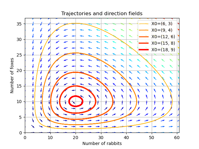
The literature contains many examples of using this model to formulate optimal control problems. See for instance Numerical Methods for Optimal Control. Our example is simpler, but it is still a hard optimization problem.

At first glance, Python may seem better suited for visualizing and exploring ODEs than for optimization. That concern is reasonable. Python is slow unless you can move most of the work into optimized library code, often implemented in C++ or accelerated with Numba. The F8 example below shows that it can be worth implementing ODEs outside Python when speed matters. For this example, however, we define the fitness function with scipy’s scipy.integrate.ode applied to the Lotka-Volterra equations. The newer scipy.integrate.solve_ivp is less suitable here for several reasons:

solve_ivp adds computation overhead, which matters when a fitness function is called many million times.
scipy.integrate.ode shows that many integrators are not reentrant. That means they cannot be used with optimization methods that rely on parallel retry or parallel function evaluation. We configure the integrator as "dopri5" and relax the accuracy requirements to speed up integration.

See lotka.py for the complete example code.

The rabbit and fox populations are propagated using:

def lotkavolterra(t, pop, a, b, c, d):
    x, y = pop
    return [a*x - b*x*y, -c*y + d*x*y]

Let us extend the rabbit/fox scenario:

We use the same initial conditions: 10 rabbits and 5 foxes.
Each year we may decide whether to hire a fox hunter.
Only one fox can be killed each year, but there must be at least one fox left after that.
For each year we can freely decide when to hunt - or to leave the foxes alone.

We follow these rules for 20 years. Then we stop hunting and observe the rabbit population for the next 5 years. The goal is to maximize the peak rabbit population during that period. The fitness function works as follows:

As input we use a vector of 20 values between -1 and 1 representing the first 20 years.
A value < 0 indicates: No hunting this year
A value >= 0 means: The value represents the fraction of the year after we kill a fox.

We first derive a list of fox kill times ts from the argument vector. Then we propagate the population between those times and kill one fox after each propagation. Finally we propagate from year 20 to year 25 to determine the maximal rabbit population in that interval:

# maximal rabbit population after dim years of fox killings
def fitness(X):
    ts = []
    for year, x in enumerate(X):
        if x > 0: # should we kill a fox this year?
            ts.append(year + x) # when exactly?
    I = integrator()
    I.set_initial_value(pop0, 0)
    for i in range(len(ts)):
        pop = integrate(I, ts[i]) # propagate rabbit and fox population to ts[i]
        pop[1] = max(1, pop[1]-1) # kill one fox, but keep at least one
        I.set_initial_value(pop, ts[i])
    # value is maximal rabbit population during the following 5 years without fox killings
    return -max([integrate(I, t)[0] for t in np.linspace(dim, dim + 5, 50)])

Let us first check the trivial solutions:

    print("shoot no fox at all, fitness = ", fitness([-0.5]*dim))
    print("shoot a fox every year, fitness = ", fitness([0.5]*dim))

resulting in:

shoot no fox at all, fitness = -40.588063495451664
shoot a fox every year, fitness = -62.19130394089944

Intuitively, killing a fox each year should maximize the final rabbit population. Let us see whether optimization can improve on the -62.19 result, and by how much:

Smart parallel retry

def smart_retry(opt = De_cpp(1500)):
    return return advretry.minimize(fitness, bounds, optimizer=opt, num_retries=50000, max_eval_fac=20)

The two algorithms to try first with smart retry are de_cma, a sequence of differential evolution and CMA-ES, and De_cpp, pure differential evolution. Our recommendation is to try de_cma for space flight dynamics problems and De_cpp in most other cases. De_cpp(1500) means each retry starts with 1500 evaluations. The maximum number of evaluations is max_eval_fac*1500 by the end of num_retries optimization runs. The result of each run is used to configure the bounds for future runs.

Parallel retry

def parallel_retry(opt = Bite_cpp(100000, M=8)):
    return retry.minimize(fitness, bounds, optimizer=opt)

The three algorithms to try first with parallel retry are Bite_cpp using "BiteOpt = BITmask Evolution OPTimization", De_cpp, pure differential evolution, and de_cma, a sequence of differential evolution and CMA-ES. This differs from the recommendation for smart retry. BiteOpt recently got a significant "boost" after being included in the fcmaes library. It became the recommended algorithm for parallel retry and as a standalone optimizer. For smart retry it still works well, but often not as well as de_cma and De_cpp.

Parallel function evaluation

def parallel_eval(opt = DE(dim, bounds)):
    return opt.do_optimize_delayed_update(fun=fitness, max_evals=500000)

The two algorithms to try for parallel function evaluation are DE and Cmaes. These are Python implementations of differential evolution and CMA-ES, and they are currently the only fcmaes algorithms that support parallel function evaluation. Try DE first, since Cmaes works well only in specific domains. You can see this yourself on the Lotka-Volterra control problem.

For the Lotka-Volterra control problem, the best approach is smart parallel retry with De_cpp. On an AMD 16 core 5950x, you can get results below -120 after about 20 seconds. -129 is reached after about 3 minutes. The final result we obtained was fitness < -132.26.

solution = [0.7764942271302568, 9.831131324541304e-13, -0.4392523575954558, 0.9999999991093724, 0.9999999993419174, 0.877806604524956, -0.21969547982373291, 0.9877830923045987, 0.21691094924304902, -0.016089523522436144, 1.0, 0.7622848572479829, -0.0004231871176822595, -0.015617623735551967, -0.9227281069513724, 0.8517521143397784, 8.397851857275901e-19, 1.0, 1.0, 0.1509108812092751]

print("best solution, fitness =", fitness(solution))

best solution, fitness = -132.261620475498

This is much better than killing a fox each year (-62.19 rabbits). Try other algorithms too, for instance scipy.minimize, algorithms from pygmo, or NLOpt. If you find an algorithm that improves on the given solution, please send me a message.

Parallel function evaluation may be an alternative. You may reach values below -125 quickly, but only if you are very lucky. Most of the time, one retry is simply not enough to solve this problem. The fcmaes DE implementation has an unusual feature: it re-initializes individuals based on their age. Because of this, the search does not get completely stuck at a local minimum, and improvements may still appear even after millions of function evaluations.

F8

The example f8.py is a new implementation of the F-8 aircraft control problem F-8_aircraft. The goal is to control an aircraft in a time-optimal way from an initial state to a terminal state.

It contains the ingredients needed for your own optimization projects with differential equations in the context of parallel retries. The example is described in detail in Oracle Penalty: In 8 hours on a PC with 2 GHz clock rate and 2 GB RAM working memory, back in 2010, the equality constraints could not be solved completely using the oracle penalty method. We use a fixed penalty weight instead.

How to implement differential equations in Python

Integrating differential equations inside the objective function is costly. It is worth doing everything possible to reduce that cost. Scipy provides two interfaces, ode and solve_ivp. For F8 we provide an ode based implementation for comparison, but we recommend compiled ODEs based on the Ascent library, see ascent.cpp Using this approach, you can get a good solution in less than a second on a fast 16 core machine.