Designing a Card Game
The code for this tutorial is at top_trumps.py. It uses retry.py and moretry.py.
The main question is this:
If we have an expensive simulation-based fitness function with several variants and only a limited evaluation budget, how should we compare optimization algorithms?
a) Test all variants at once with a very small budget, single-threaded. b) Test all variants in parallel. c) Choose one variant and test it with multiple retries in parallel.
With modern many-core CPUs, option a) is easy to rule out. Option b) breaks down when algorithms scale differently as the evaluation budget grows. In that case, low-budget results do not predict high-budget performance. Option c) fails if algorithm rankings change strongly across problem variants.
A fair comparison should therefore consider both approaches. Approaches a) and b) are already covered by coco-gbea and its associated competitions, so we start here with approach c).
If the algorithms favored by c) differ from those favored by b), which ones are better for real-world use?
This tutorial shows:
-
How parallel
fcmaessingle-objective optimizers can be used to design a TopTrumps card deck. -
How
fcmaessingle-objective optimizers, together with a specialized parallel retry implementation, can efficiently approximate the pareto front of related multi-objective problems. -
That optimization algorithms scale differently as the evaluation budget increases.
-
How budget management affects optimizer performance.
-
How the well-known ERT (Expected Running Time) metric influences optimizer design, and why that may not align with hard real-world problems.
UPDATE
fcmaes now includes the multi-objective algorithm MO-DE, which also supports constraints. This tutorial predates that addition. For the multi-objective variant discussed here, MO-DE is now the preferred method.
top_trumps.py has been updated and shows how to call both the Python and the C++ variants. Try its nsga_update parameter to see which setting fits best. For this problem, nsga_update=False, which uses the DE update method, works better. It is also better than all other methods presented here.
Since this is a mixed-integer problem, you can also use the ints parameter to specify the discrete parameters. If you do that, adapt the bounds to integer values.
coco-gbea
coco-gbea is derived from the black-box optimization test project coco. It adds Game Benchmarks for Evolutionary Algorithms (GBEA), described in detail in Single- and multi-objective game-benchmark for evolutionary algorithms. We focus on the TopTrumps benchmarks here for several reasons:
-
They provide an efficient reentrant C implementation of several game-design fitness functions, some of them based on game simulation.
-
Even in larger dimensions that reflect realistic game scenarios, the fitness function is still fast to evaluate.
-
The suite contains both single-objective and bi-objective problems. For the bi-objective cases, the objectives were selected carefully based on estimated conflict using linear regression.
-
The benchmark is well suited to demonstrate how optimizers scale with budget, and how budget management matters in parallel optimization.
-
It is also a good setting for discussing ERT (Expected Running Time) as a performance metric, because it exposes its weaknesses clearly.
Some parts of the TopTrumps test environment are less useful if your goal is to solve the TopTrumps problems efficiently:
-
The original setup uses a socket-based interface to call the C fitness function single-threaded. You need a separate port for each parallel run, and this adds unnecessary overhead. Sockets or a REST interface make sense when distributing work across machines, but not for local execution.
-
The design is strongly influenced by ERT. Under that metric, there is little incentive to support parallel access to the fitness function itself.
The socket interface can be replaced in Python with a much simpler ctypes interface, because rw_top_trumps.cpp exposes the fitness functions (evaluate_rw_top_trumps) as extern "C"rw_top_trumps.cpp is reentrant, the interface implemented in
top_trumps.py
supports parallel execution.
Expected Running Time
From Optimization Benchmarking, page 24:
"The gold standard in (single-objective) continuous optimization is the Expected Running Time (ERT), which computes the ratio between the sum of consumed budget across all runs and the number of successful runs Hansen.et.al 2012".
Unfortunately, this definition does not match what many users expect from something called "running time". ERT measures budget, not elapsed time. On older single-core systems, time and budget were more closely related. Today even standard desktop machines have 16 cores and 32 threads, and cloud machines with 64 cores and 128 threads are easy to rent. To judge whether the ERT "gold standard" is convincing, consider these questions:
-
A parallel optimization algorithm increases the evaluation rate per second by a factor of 20, but needs 20% more evaluations to reach a given threshold. Do you use parallelization?
-
You found a surrogate model that is 100 times faster to evaluate than the original model, but it needs 20% more evaluations to reach the same threshold. Do you use the surrogate?
-
You can choose between two algorithms. The second has a 20% better ERT, but much higher overhead, so wall-clock time is worse even with the smaller budget. Do you still choose the second one?
-
Does it matter where parallelization is applied: inside the fitness function, over a population, across retries of the same experiment, or across separate experiments?
-
You provide a benchmark suite with an expensive simulation-based fitness function that is evaluated millions of times. By default, do you compile the simulation with
-O2? Do you design the simulation server to evaluate fitness in parallel, or is it enough to run multiple experiments in parallel?
The ERT "gold standard" ignores evaluation rate, meaning how many evaluations can be completed in a given time. A more intuitive alternative is "real running time" (RRT): the actual time needed to reach a threshold, including algorithm overhead and the effect of parallelization. Its drawback is that it depends on the available hardware. Still, as the examples below show, ignoring overhead and parallelization entirely is usually the worse choice.
You may ask whether ERT and RRT are equivalent for a fixed machine and a fixed level of parallelization.
-
They are equivalent for one specific optimizer only: random search. For more serious algorithms they differ, for several reasons:
-
The evaluation rate depends on how parallelization scales, and that depends on what exactly you parallelize: the fitness function, a whole population, retries of one experiment, or complete experiments.
-
If an algorithm relies on retries, the best budget allocation and algorithm choice can change in a parallel setting when the goal is to minimize RRT.
-
Parallel retries may exchange information. See, for example, the pagmo archipelago topology.
In the end, you have to decide whether you tune a parallel optimizer for ERT or for RRT on a specific CPU. An ERT-tuned algorithm will usually have worse RRT, and the reverse is also true. Both choices are valid:
-
You want to win the gbea competition, or another coco-based competition: tune for ERT.
-
You want to solve a real-world optimization problem because you need the result. For TopTrumps, that means producing an exciting card game: tune for RRT.
Even if your goal is ERT, you should still ask whether a full coco suite with a low budget factor is the right starting point. That strategy is similar to a breadth-first search, and it only makes sense if two conditions hold:
-
Low-budget results let you predict algorithm performance at higher budgets.
-
You expect different fitness functions in the suite to favor different algorithms.
If those conditions do not hold, a depth-first strategy is better. Pick a representative problem and try to solve it, even if that requires a large budget. If an algorithm cannot solve that example, discard it and move on. This keeps algorithms that look slow at low budgets but scale well later. Random search is often overrated when the test budget is small. Deep BITmask Evolution OPTimization BiteOpt, by contrast, can easily be underrated by an ERT benchmark. It needs more budget, but scales much better and diversifies effectively, which makes many parallel retries worthwhile. In many cases a single run will never reach the target threshold, no matter how much budget you invest.
TopTrumps
The gbea TopTrumps benchmark is a carefully designed real-world benchmark. Its single-objective and multi-objective fitness functions reflect actual requirements a TopTrumps card game designer might care about. The simulation-based tests are implemented efficiently, so it is practical to compare optimizers under limited CPU time, especially when parallelization is used.
To support that, I replaced the socket-based interface with a simpler ctypes interface. This was straightforward because rw_top_trumps.cpp exposes the fitness function (evaluate_rw_top_trumps) as extern "C"coco-gbea2/code-experiments/rw-problems/top_trumps yourself, add -O3 to CXXFLAGS in the Makefile, and copy the result to fast-cma-es/fcmaes/lib. The Python class tt_problem provides both bounds and the fitness function through reentrant ctypes calls to evaluate_rw_top_trumps and rw_top_trumps_bounds.
This tutorial first focuses on two specific simulation-based problem instances. The first is a single-objective case, the trick difference at the end of the game:
    suite = 'rw-top-trumps'
    function = 5
    instance = 5
    dim = 128
    nobj = 1
    name = suite + '_f' + str(function) + 'i' + str(instance) + 'd' + str(dim)

    problem = tt_problem(suite, name, dim, nobj, function, instance)
The second is a bi-objective case with competing objectives: win rate of the better player and switches of trick winner:
    suite = 'rw-top-trumps-biobj'
    function = 2
    instance = 5
    dim = 128
    nobj = 2
    name = suite + '_f' + str(function) + 'i' + str(instance) + 'd' + str(dim)
problem = tt_problem(suite, name, dim, nobj, function, instance)-
The simulation-based functions are noisy. However, the fitness for each solution is reported as the average of 2000 simulations, which has been shown in to produce an appropriate balance between computational effort and resulting standard deviations. This shows a typical property of real world fitness functions:
For the model used for optimization, there is a tradeoff between accuracy and computational effort. That means the pareto front you get from the optimization model is not necessarily the final one you care about. Suppose the algorithm returns good but slightly dominated solutions like these:
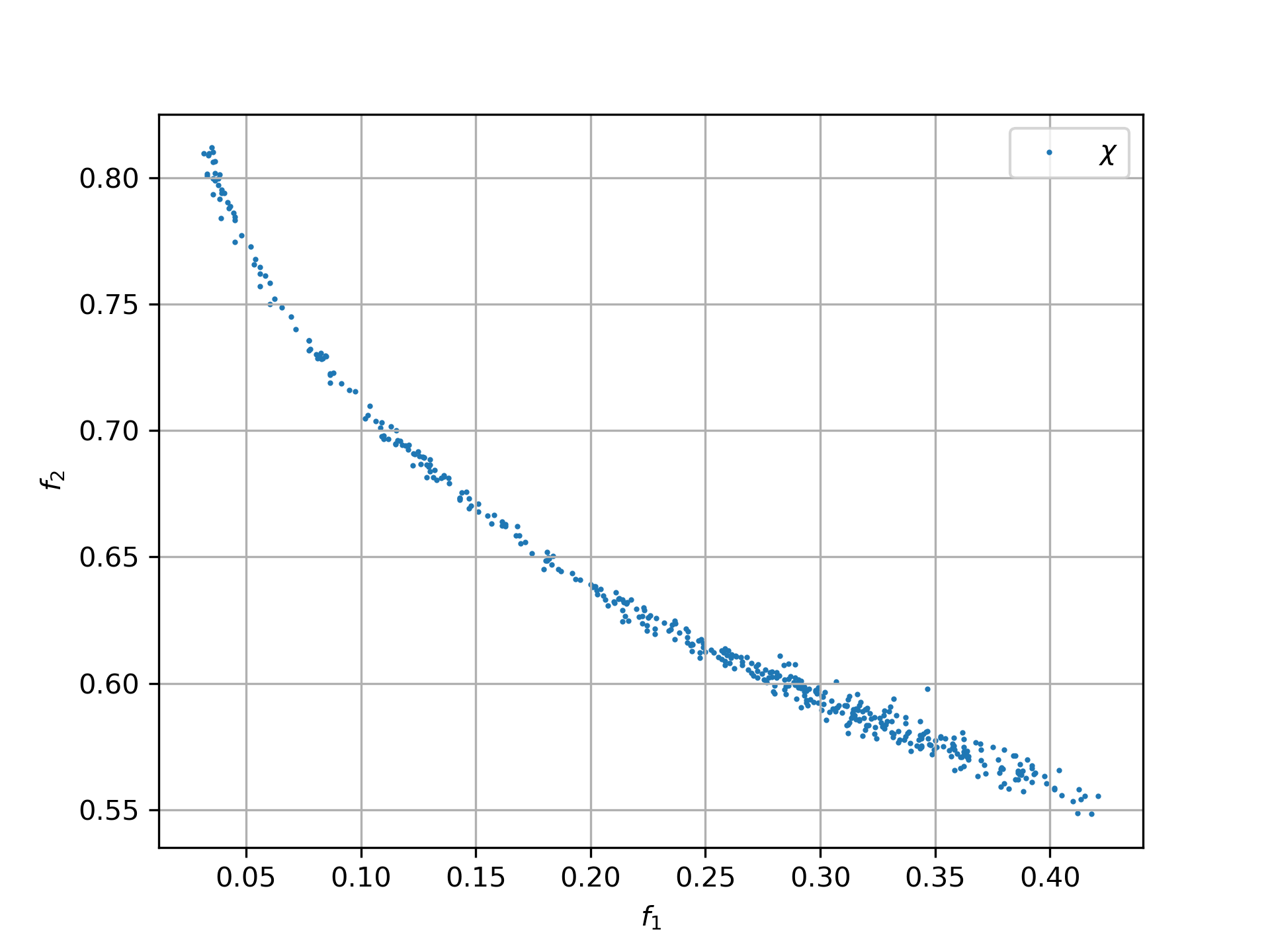
You can then reevaluate the small set of solution vectors with a more accurate model and compute the pareto front only after that. A point that looked slightly dominated before may become non-dominated. For TopTrumps this may not matter much, but for other real-world problems it can matter a lot. Some expensive objectives or constraints may have been omitted entirely, or the constraints may have changed after a long simulation-based optimization run finished.
The fcmaes library provides convenience functions for testing parallel optimizers. These functions produce both a detailed log file and plots that show progress over time or the resulting pareto front.
from fcmaes.optimizer import de_cma, Bite_cpp, Cma_cpp, De_cpp, random_search, wrapper
from fcmaes import moretry, retry

def mo_minimize_plot(problem, opt, name, exp = 3.0, num_retries = 256):
    moretry.minimize_plot(name, opt, wrapper(problem.fun), problem.bounds, problem.weight_bounds,
                          num_retries = num_retries, exp = exp)

def minimize_plot(problem, opt, name, num_retries = 256):
    retry.minimize_plot(name, opt, problem.fun, problem.bounds,
                          num_retries = num_retries)
At this point fcmaes does not use dedicated multi-objective algorithms here. Instead, it runs single-objective optimizers in parallel with a weighted-sum approach and random weights. That often works surprisingly well, especially when the alternative is a single-threaded dedicated MO algorithm. For many real-world multi-objective problems from space-flight planning with multiple gravity assists, it is the only approach that works.
Here are typical optimizer configurations for the chosen single-objective problem variant:
    budget = 4000
    retries = 64
    minimize_plot(problem, random_search(budget), name + '_10k64', num_retries = retries)
    minimize_plot(problem, Cma_cpp(budget), name + '_10k64', num_retries = retries)
    minimize_plot(problem, De_cpp(budget), name + '_10k64', num_retries = retries)
    minimize_plot(problem, Bite_cpp(budget, M=16), name + '_10k64', num_retries = retries)
And here are the configurations for the multi-objective problem variant. More retries are needed because the pareto front is generated from random weights.
    budget = 4000
    retries = 512
    mo_minimize_plot(problem, random_search(budget), name + '_4k512', num_retries = retries)
    mo_minimize_plot(problem, Cma_cpp(budget), name + '_4k512', num_retries = retries)
    mo_minimize_plot(problem, De_cpp(budget), name + '_4k512', num_retries = retries)
    mo_minimize_plot(problem, Bite_cpp(budget, M=16), name + '_4k512', num_retries = retries)
All experiments were performed on the same processor, a 16-core AMD 5950x using 32 parallel optimization retries.
TopTrumps single-objective function 5, instance 5, dim = 128, 10000 evaluations, 64 retries
-
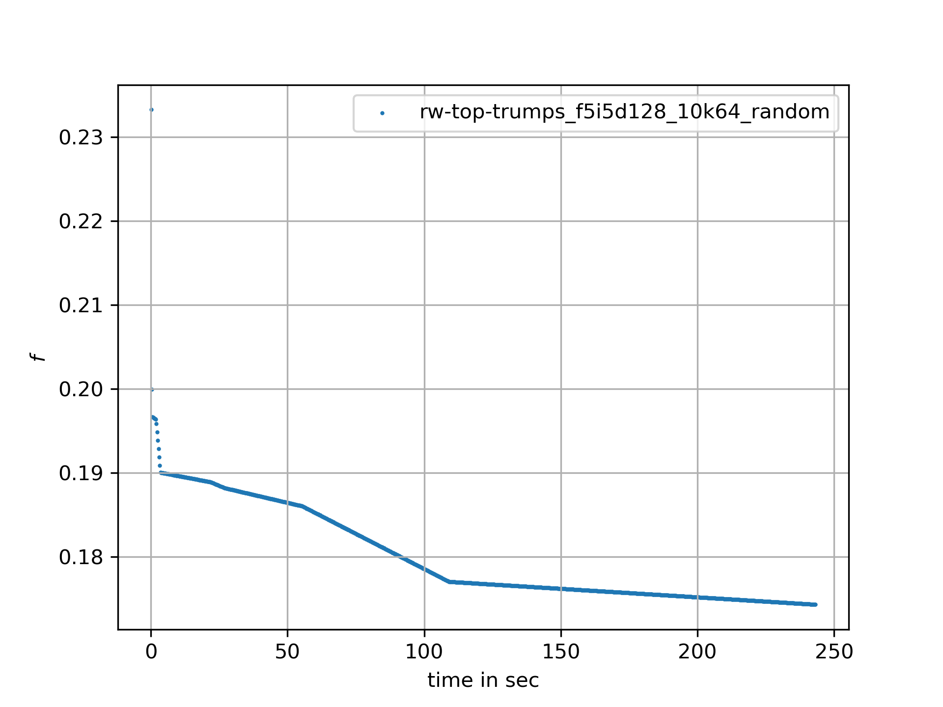
Random search
Even a budget of 64 * 10000 = 640000 evaluations is not enough to find good solutions. But note that after 20 seconds, about 6000 evaluations, random search is better than all other optimizers. You should never judge an optimizer after only a few evaluations.
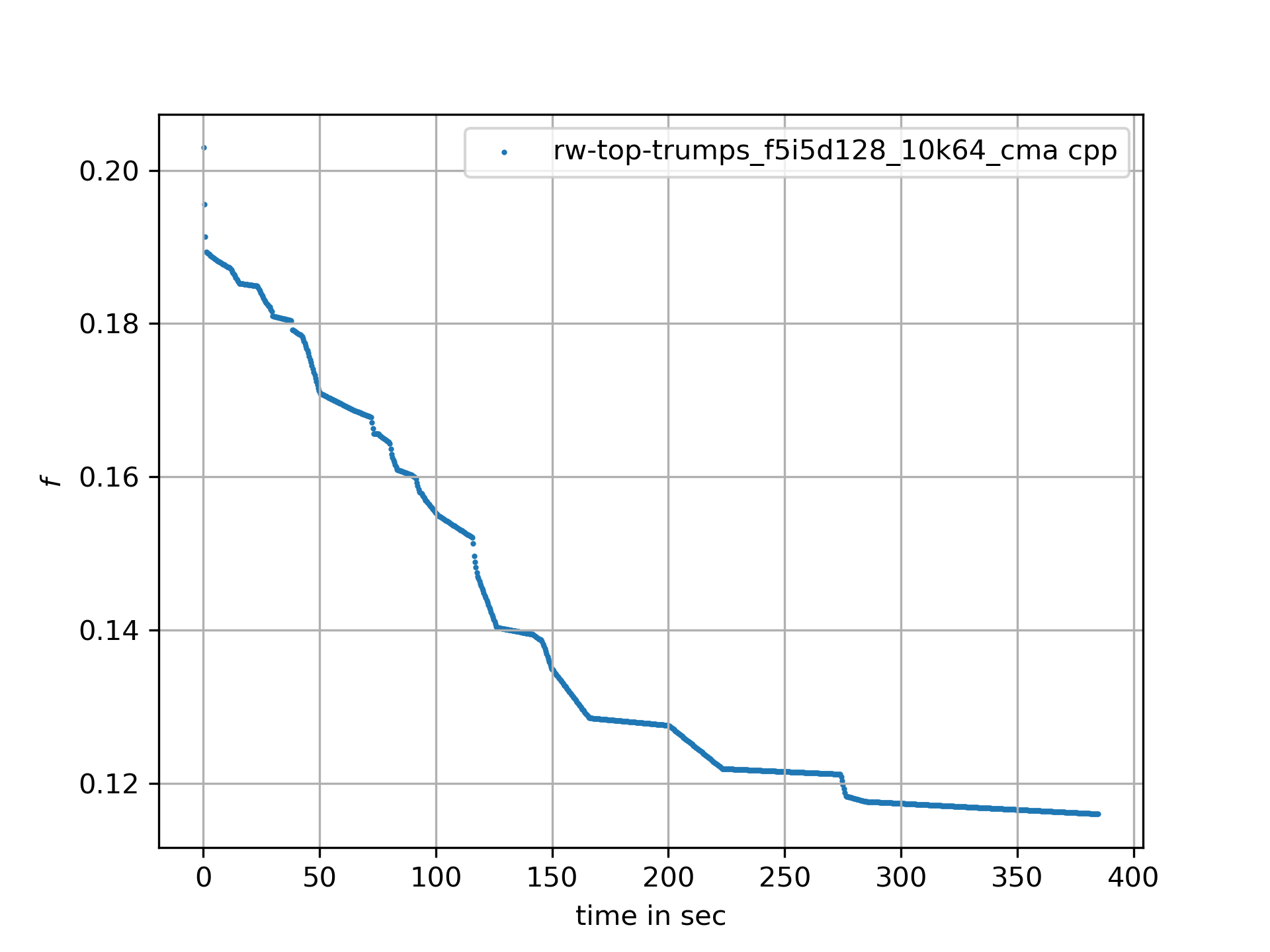
CMA-ES performs better overall. It reaches its best result, around 0.117, after about 400 seconds, but then stops improving.
-
CMA-ES, popsize = 31
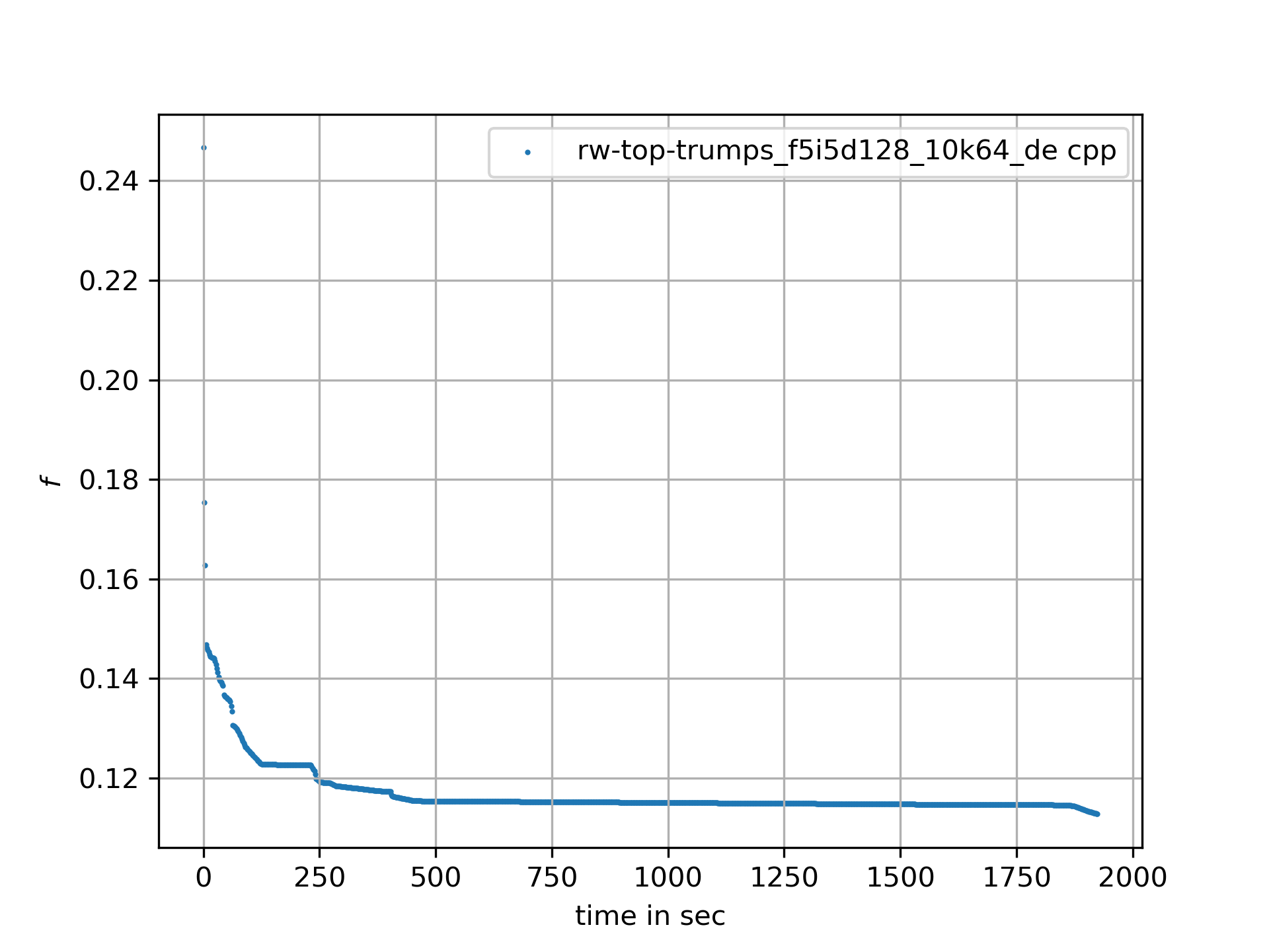
The fcmaes differential evolution variant (DE) crosses 0.12 after about 250 seconds, similar to CMA-ES. Unlike CMA-ES, it still finds a later improvement and ends around 0.113.
-
DE, popsize = 31
Deep Bite optimization (BiteOpt) is the clear winner here. It crosses 0.10 after about 600 seconds and improves further to 0.0959 after about 1200 seconds.
-
Deep Bite optimization, M=16
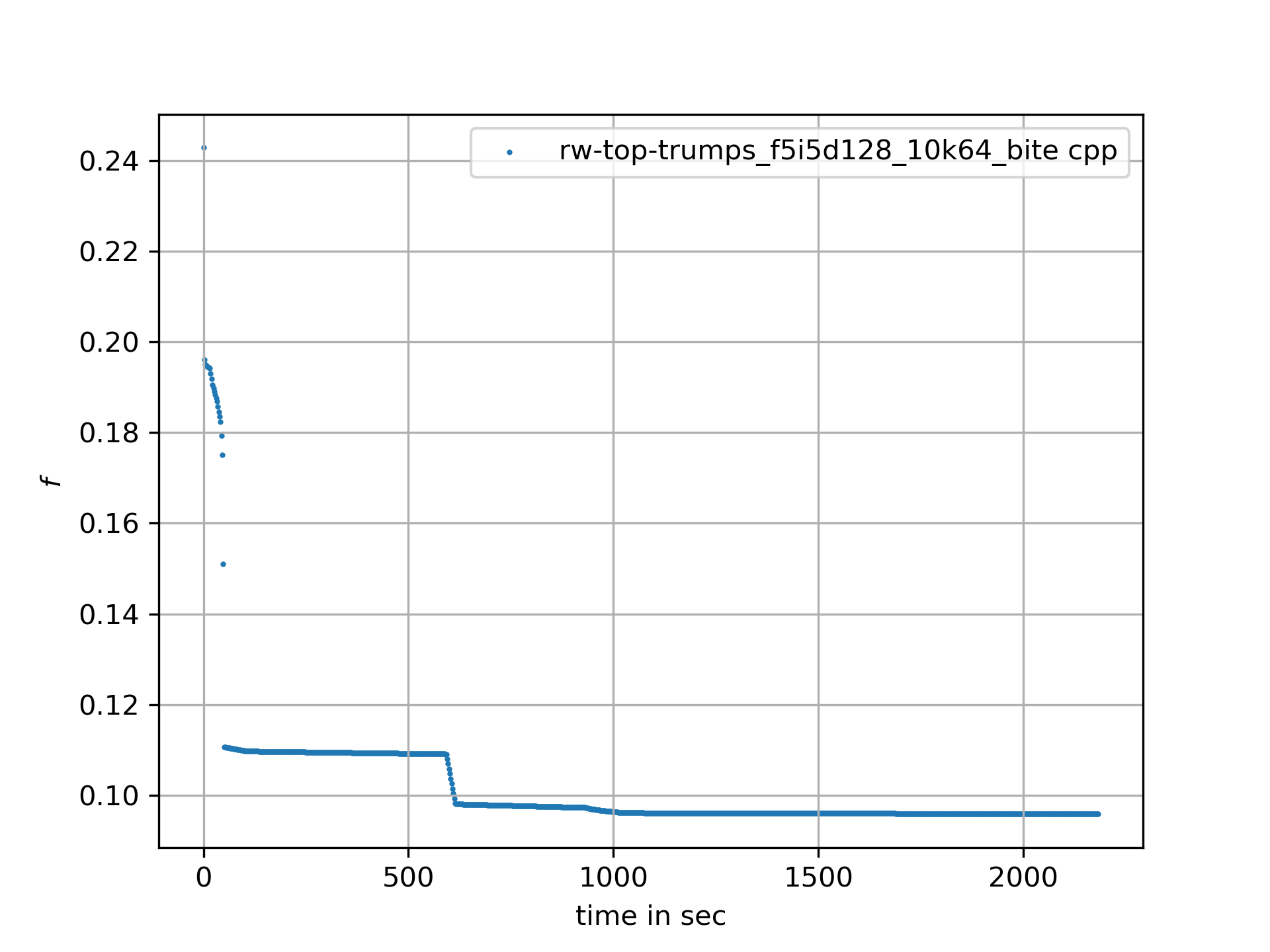
Here is the best solution found by the BitOpt algorithm after about 1200 seconds on a 16-core CPU executing 32 optimizations in parallel:
x = [16.0, 54.0, 12.0, 36.0, 16.0, 54.0, 12.0, 36.0, 16.0, 54.0, 11.0, 36.0, 16.0, 54.0, 12.0, 36.0, 16.0, 54.0, 12.0, 36.0, 16.0, 54.0, 12.0, 36.0, 16.0, 54.0, 12.0, 36.0, 16.0, 54.0, 12.0, 36.0, 16.0, 54.0, 12.0, 36.0, 16.0, 54.0, 12.0, 36.0, 16.0, 54.0, 12.0, 36.0, 16.0, 54.0, 12.0, 36.0, 16.0, 54.0, 12.0, 36.0, 16.0, 54.0, 12.0, 36.0, 16.0, 54.0, 12.0, 36.0, 16.0, 54.0, 12.0, 35.0, 16.0, 54.0, 12.0, 36.0, 16.0, 54.0, 12.0, 36.0, 16.0, 54.0, 12.0, 36.0, 16.0, 54.0, 12.0, 36.0, 16.0, 54.0, 12.0, 36.0, 16.0, 54.0, 12.0, 36.0, 16.0, 54.0, 12.0, 36.0, 16.0, 54.0, 12.0, 36.0, 16.0, 54.0, 12.0, 36.0, 16.0, 54.0, 12.0, 36.0, 16.0, 54.0, 12.0, 36.0, 16.0, 54.0, 12.0, 36.0, 16.0, 54.0, 12.0, 36.0, 16.0, 54.0, 12.0, 36.0, 16.0, 54.0, 12.0, 36.0, 16.0, 54.0, 12.0, 36.0]

y = problem.fun(x) = 0.095875
This result shows an almost perfect repeated pattern. That suggests trying a reduced 4-dimensional formulation by repeating the same four arguments across the full vector. In fact, many repeated patterns produce a good result around 0.098, but 0.0958 seems unreachable that way.
TopTrumps bi-objective function 2, instance 5, NGSA-II, 4000 generations, popsize = 200
For the bi-objective problem with competing objectives, win rate of the better player and switches of trick winner, let us first try the well-established NGSA-II algorithm. We use a single-threaded implementation, so the optimization took about 17.3 hours.
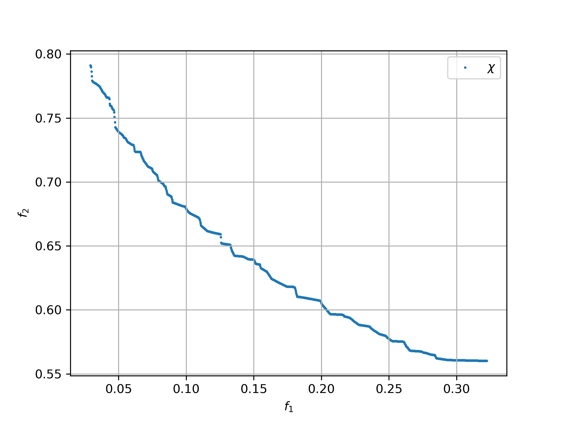
TopTrumps bi-objective function 2, instance 5, dim = 128, 4000 evaluations, 512 retries, pareto front
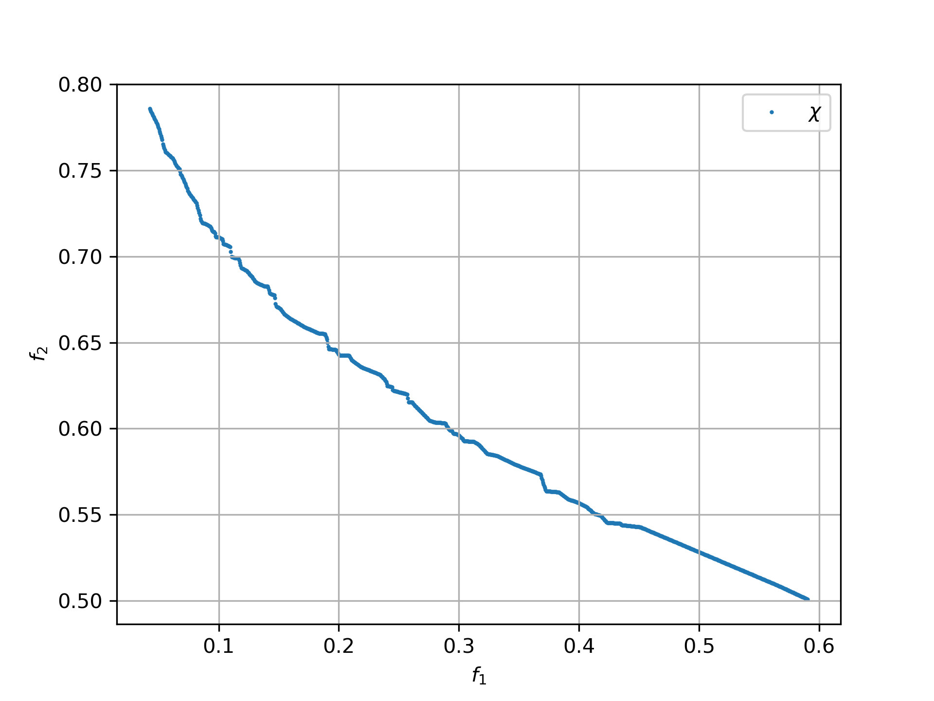
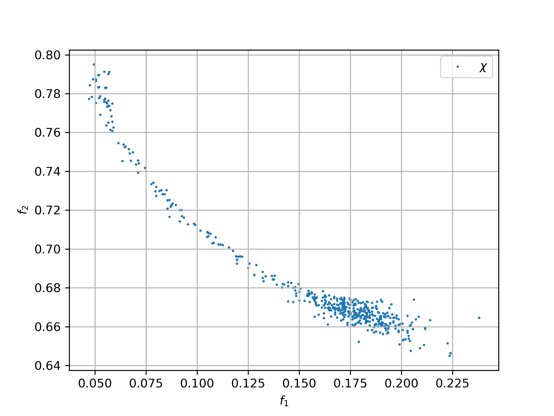
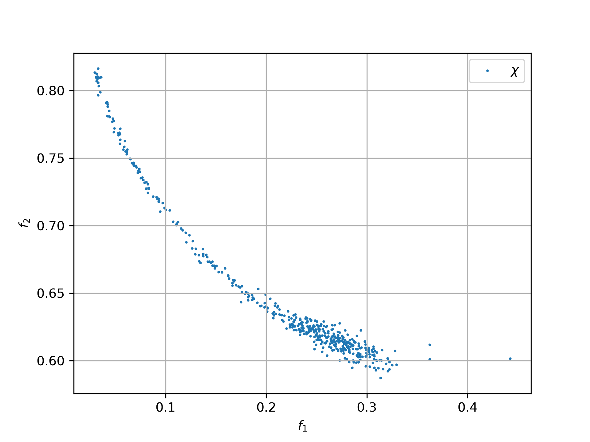
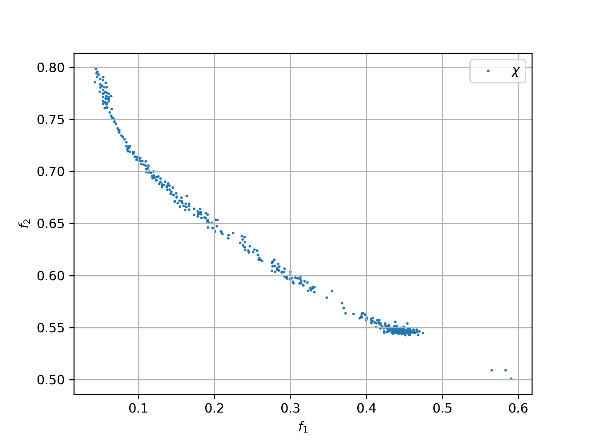
Here the evaluation budget increases to 4000*512 function calls, compared to the 4000*200 calls used for NSGA-II. Even so, each test took only about 2.2 hours. The reason is the strong scaling from running 32 optimizations in parallel on the 16-core AMD 5950x CPU. As expected, random search is worse than NGSA-II:
-
Random search
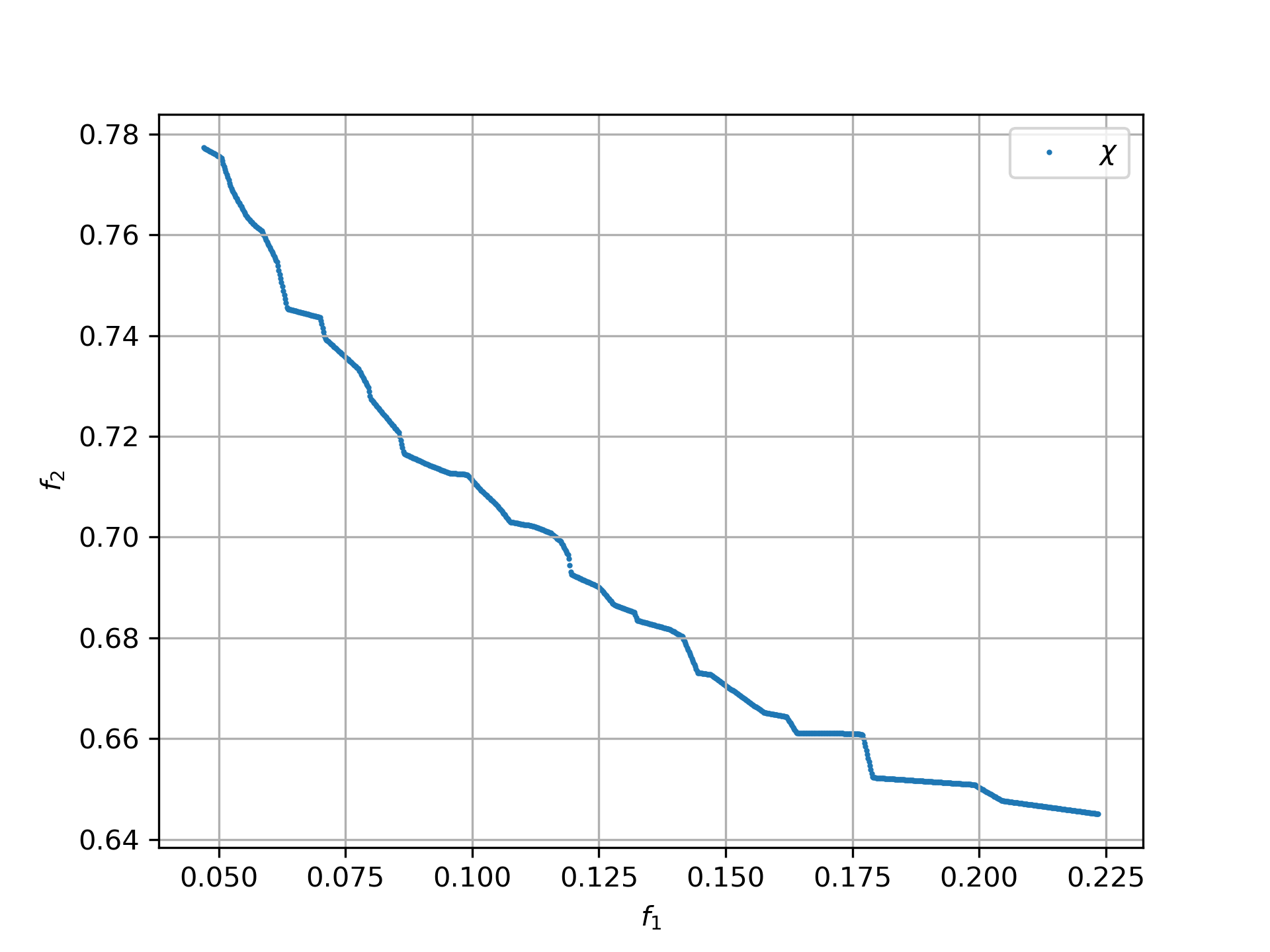
-
CMA-ES, popsize = 31
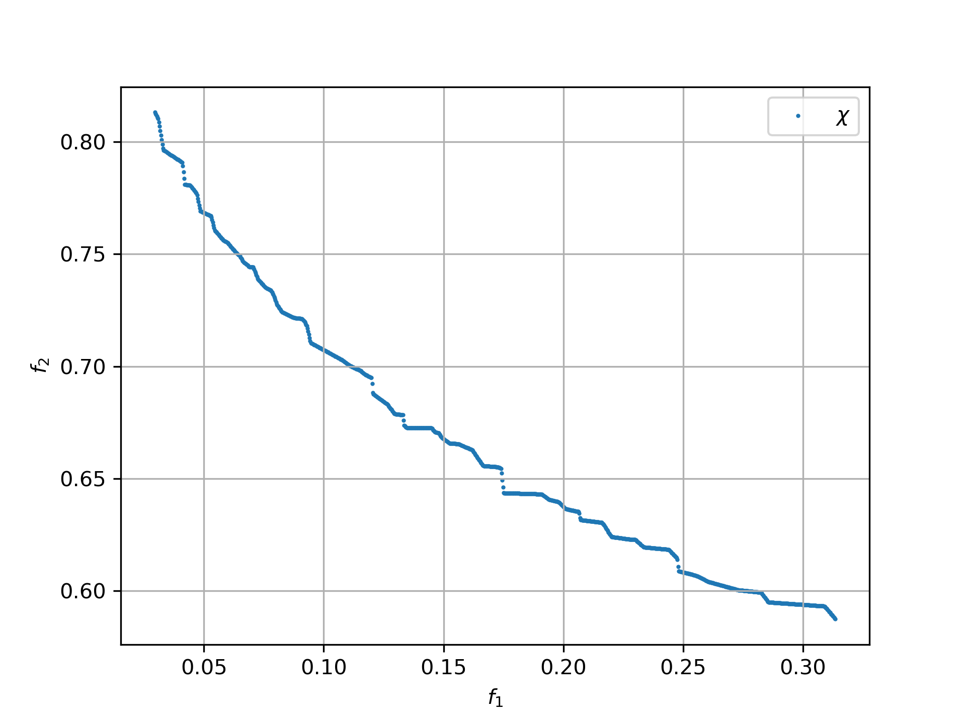
-
DE, popsize = 31
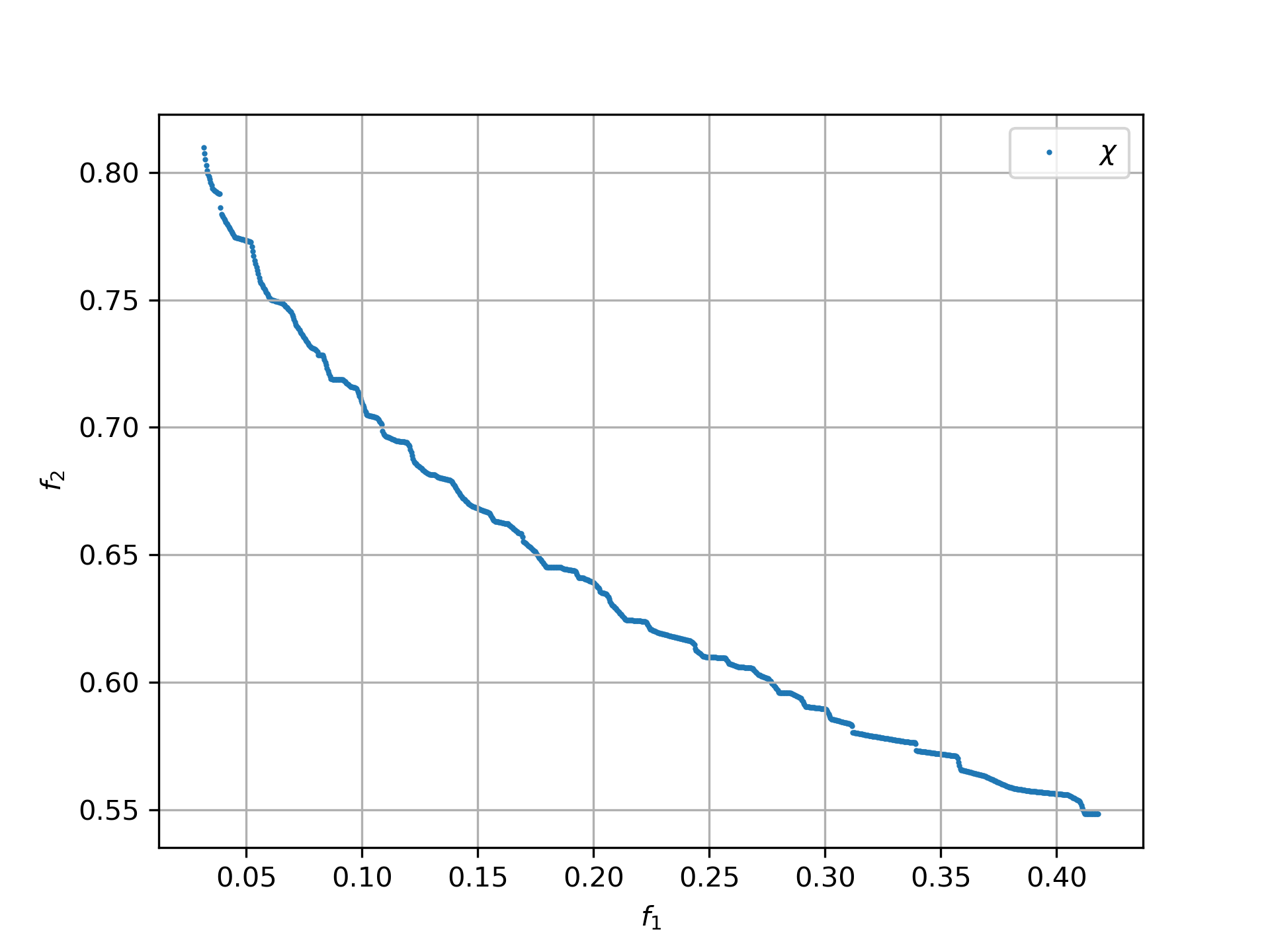
BiteOpt finds significantly better results for the second, simulation-based objective:
-
Deep Bite optimization, M=16