

Analyzing Social Media User Data
This tutorial
-
shows how to analyze social media user data, including friend and group relations between users, using an adapted multi-objective version of the vertex cover optimization problem.
-
shows how to solve the vertex cover problem using
-
The Python jgrapht graph library.
-
An improved greedy algorithm.
-
By continuous optimization
-
-
explains why you should not apply continuous optimization to the vertex cover problem.
-
shows that the insights gained from solving vertex cover by optimization may help with real-world coverage-related problems.
The code for this tutorial is here:
Motivation
The vertex cover problem is one of the most studied combinatorial problems in computer science. There are countless publications and algorithms. Recent work even includes deep learning approaches (see https://arxiv.org/pdf/1810.10659.pdf and https://www.youtube.com/watch?v=XVLd7hf6y6M ).
So why add another implementation, especially one that will perform poorly on the classic problem? Because the real interest here is not the textbook variant. Real-world problems related to vertex cover are often less studied, and standard greedy algorithms cannot always be adapted to them. If we frame the task as an optimization problem, vertex cover becomes easier to extend to these settings.
If you have not watched The great Hack yet, this is a good time. It is closely related to the scenario discussed here. The movie is about the use and misuse of social media user data for targeted political influence campaigns. There are also legitimate uses for this kind of data, for example targeting advertisements to users who are likely to spread information further through friends and groups.
We will use anonymised Facebook user relation data. That is enough to demonstrate the idea. The data is described and analyzed in http://i.stanford.edu/~julian/pdfs/nips2012.pdf .
Constraint Programming and Optimization
Constraint Programming is a very popular way to solve combinatorial problems. Vertex cover is a typical example, because the constraint is simple: all edges must be covered. But that changes if we are not only interested in fully feasible solutions. Instead, suppose we want to study the tradeoff between investment (here: the number of selected vertices) and ROI, return on investment (here: the proportion of fulfilled constraints). Then the problem becomes a (multi-objective) optimization problem, and we need different tools. This is true even before considering that the number of constraints can explode in practice. Large fully connected subsets of vertices are enough to cause that.
Exercise: How many edges do we get from a fully connected subset of 1000 vertices?
Recently it has become popular to apply deep reinforcement learning to combinatorial problems. That still does not address cases where the tradeoff itself matters more than a complete solution.
Continuous optimization is a natural fit once we focus on the desired result: an optimal tradeoff, or in the multi-objective case, a set of non-dominated solutions.
Instead of accumulating thousands of constraints, we define a fitness function that computes the proportion of fulfilled constraints. For vertex cover this is equivalent to counting the number of uncovered edges. This also lets us assign different weights to uncovered edges and selected vertices. As we will see later, that often makes sense in real applications.
How does an optimizer work? It proposes solutions and gets their fitness as feedback. From that feedback it generates better proposals, and the process repeats. For each evaluation we need to count the number of unfulfilled weighted constraints. We do not need to store them in memory, unlike CP, but we still need to count them. Whether this approach is feasible depends on how fast that counting step is. We use parallel execution and numba to speed it up dramatically.
To give a concrete number for the example below: We count 30025 edges / constraints on average 405582 times per second on an 16 core AMD 5950x processor. This is 1.218E10 counts per second. This includes the computational overhead of the optimizer itself. Even if we need 1E7 fitness evaluations / 3E12 counts to find a good solution, this still means less than 30 seconds wall time.
What about the decision variables? Combinatorial problems require discrete input. There are several ways to convert continuous variables into discrete decisions:
-
You need a subset selection of a set of n elements: map n decision variables x_i in the [0,2] interval by x_i >= 1 → "is in" and x_i < 1 → "is out".
-
You need a specific ordering of n elements: map n decision variables X in the [0,1] interval to numpy.argsort(X) - use the disjoined indexes of the sorted list.
-
You need a list of size m out of n elements: map m decision variables x_i in the [0,n] interval by x_i → int(x_i).
Vertex coverage requires the first mapping. We select a subset of n vertices.
We often underestimate what modern processors can do for counting and optimization, and overestimate what they can do for constraint programming. In particular, we tend to underestimate memory limits. See also link:Clustering.html where we describe a combinatorial clustering problem that scales very badly with CP. Optimization is much easier to parallelize. Because of the current machine learning hype, we also tend to overlook how many parallel operations deep learning uses internally. The same move to multi-core architectures that enables machine learning also enables continuous optimization in domains where it may seem unexpected.
Scenario
Suppose we want to run a targeted campaign to influence people, and we have user data that describes their relationships. People may be linked directly as friends or indirectly through groups. Some people are easy to influence, others are hard. Assume we have a rough normalized cost estimate in [0,1] for each person. The sum of these costs gives an upper bound on what we can invest. Our goal is to minimize cost and maximize impact by influencing the right people and using their friend and group relationships.
As a first approximation, we can model people as graph nodes and friendship relations as graph edges. Then we can apply vertex cover to find the smallest set of people connected to the full population. This model has several flaws:
-
It ignores group relations. We could transform groups into additional edges, but this scales poorly because the number of edges grows quadratically with group size. It also raises another question: should group relations be weighted differently depending on group size?
-
It ignores the different costs of influencing different people. There is a related weighted vertex cover variant.
-
It may return high costs or a large set of people because it ignores solutions with less than 100% coverage, even though these may be valid alternatives.
What we really need for an investment decision is a list of non-dominated solutions. Each solution should represent a different investment level together with the corresponding best set of people to influence. In other words, we need a pareto front for a multi-objective problem where cost and impact or coverage compete.
Solving the Vertex Cover Problem in Python
Let us start with the easy variant: no groups, no vertex weights, and full edge coverage only.
Using jgraptht
We found and adapted a solution here
utils.py.
jgrapht is a Java library with a Python front end. It is very fast, but the result has some error.
def nx_to_jgraph(g):
    import jgrapht
    jg = jgrapht.create_graph(directed=False, weighted=False,
                             allowing_self_loops=False, allowing_multiple_edges=False)
    jg.add_vertices_from(list(g.nodes))
    jg.add_edges_from(list(g.edges))
    return jg

def solve_jg(g):
    import jgrapht
    jg = nx_to_jgraph(g)
    start_time = time.time()
    mvc = jgrapht.algorithms.vertexcover.greedy(jg)
    #mvc = jgrapht.algorithms.vertexcover.edgebased(jg)
    #mvc = jgrapht.algorithms.vertexcover.clarkson(jg)
    #mvc = jgrapht.algorithms.vertexcover.baryehuda_even(jg)
    mvc_size = int(mvc[0])
    print ("jgraph mvc size", mvc_size , ' of nodes: ', len(list(g.nodes())),
           ' time = ', round(time.time()-start_time, 3), ' sec')
Executing
    g = nx_graph("1912.edges")
    solve_jg(g)
results in:
jgraph mvc size 631 of nodes: 747 time = 0.021 sec
This is very fast: 0.021 sec. We get a list of 631 individuals that covers the whole population of 747 through friendship edges. But maybe this number can be reduced.
Using a greedy algorithm
This code is inspired by
SA.py.
Note that neither the improved variant shown here nor the original code actually implements
"Simulated Annealing" as stated in the original. Still, it is a very efficient algorithm and works
well even for huge graphs. It is not as fast as jgrapht.algorithms.vertexcover.greedy,
but it has a significantly lower error rate. The code also performs some statistical analysis
on the fly. It estimates the mean number of iterations needed to find an improvement and adapts
the algorithm accordingly. First, an initial solution is constructed:
def initial_solution(g):
    solution = list(g.nodes())
    # sort nodes for degree, low degree has better chance not to uncover an edge
    for _, node in \
            sorted(list(zip(list(dict(g.degree(solution)).values()), solution))):
        remove = True
        for neighbor in g.neighbors(node): # all neighbors covered?
            if neighbor not in solution:
                remove = False # bad luck, would uncover an edge
        if remove:
            solution.remove(node)
    return solution
We start with all nodes, so all edges are covered. Then we order the nodes by degree. Nodes with low degree have the best chance of being removable without breaking full coverage. We test them one by one, starting with the lowest degree nodes. If a node has a neighbor that is already outside the solution, removing it would uncover an edge. Otherwise we can remove it.
Then we try to improve the solution under a time limit.
def remove_node(g, solution, mean, start_time, max_time):
    solution = solution.copy()
    uncovered = []
    while len(uncovered) == 0:
        to_delete = random.choice(solution)
        for neighbor in g.neighbors(to_delete):
            if neighbor not in solution:
                uncovered.append(neighbor)
                uncovered.append(to_delete)
        solution.remove(to_delete)
    i = 0
    max_i = mean * 10
    while len(uncovered) > 0 and i < max_i and \
            time.time() - start_time < max_time:
        i += 1
        # delete node from solution
        next_solution = solution.copy()
        next_uncovered = uncovered.copy()
        to_delete = random.choice(solution)
        solution.remove(to_delete)
        for neighbor in g.neighbors(to_delete):
            if neighbor not in solution:
                uncovered.append(neighbor)
                uncovered.append(to_delete)
        # add node to solution
        to_add = random.choice(uncovered)
        solution.append(to_add)
        for neighbor in g.neighbors(to_add):
            if neighbor not in solution:
                uncovered.remove(neighbor)
                uncovered.remove(to_add)
        # update solution if uncovered shrink
        if len(next_uncovered) < len(uncovered) or \
            (len(next_uncovered) == len(uncovered) and \
                i > mean and random.random() < 1.0/mean):
            solution = next_solution.copy()
            uncovered = next_uncovered.copy()
    return solution, uncovered, i
We remove a random node and keep track of the nodes involved in uncovered edges. Then we try to cover those edges again by adding uncovered nodes back in random order. If that succeeds, we continue. If we spend too many attempts, relative to the observed average number of tries, we restore the node and move on.
def solve_greedy(g, seed, max_time):
    print("seed", seed)
    random.seed(seed)
    start_time = time.time()
    solution = initial_solution(g)
    iters = []
    mean = 10000
    while time.time() - start_time < max_time:
        next_solution, uncovered, i = remove_node(g, solution, mean, start_time, max_time)
        iters.append(i)
        mean = np.mean(iters)
        if len(uncovered) == 0:  # all covered ?
            solution = next_solution
            print(round(time.time()-start_time,3), len(solution), i, int(mean))

    print(round(time.time()-start_time,3), len(solution))
    print('Solution: ({}) {}'.format(len(solution), solution))
    return solution
Because these greedy improvements use random choices for removing and replacing vertices,
the method parallelizes easily. We run the same code in parallel with different random seeds
and collect the results. Since the results vary, this gives us a good chance of finding a better
solution. Note that the same graph is passed to the subprocesses, but Python multiprocessing still
uses separate graph instances. We therefore do not collect results in a shared list. Instead,
we rely on pool.starmap to gather the solutions.
def run_solve(g, max_time):
    return solve_greedy(g, random.randint(0, 100000000), max_time)

def solve_multiprocessing(g, num, max_time):
    with Pool(processes=num) as pool:
        solutions = pool.starmap(run_solve, [[g, max_time] for _ in range(num)])
    return solutions
Executing
    g = nx_graph("1912.edges")
    solve_multiprocessing(g, 10, 10)
results in:
10.001 625
Solution: (625) [415, 606, 166, 26, 148, 326, 169, 595, 503, 577, 395, 672, 668, 62, 93, 105, 635,...
10.0 625
Solution: (625) [171, 443, 301, 614, 228, 232, 594, 12, 267, 369, 45, 217, 324, 367, 47, 169, 353,...
10.0 625
Solution: (625) [514, 497, 133, 230, 368, 370, 730, 407, 487, 86, 193, 540, 669, 681, 701, 32, 562,...
10.0 625
Solution: (625) [587, 386, 130, 520, 208, 227, 196, 41, 426, 692, 485, 16, 160, 327, 557, 559, 292,...
10.001 624
Solution: (624) [737, 207, 589, 509, 571, 17, 435, 465, 443, 387, 73, 307, 510, 646, 490, 409, 507,...
10.001 623
Solution: (623) [464, 641, 558, 351, 478, 484, 563, 24, 668, 195, 519, 360, 217, 676, 405, 530, 4,...
10.0 623
Solution: (623) [14, 130, 340, 360, 491, 591, 505, 497, 64, 352, 5, 668, 114, 141, 157, 520, 606, 187,...
10.001 623
Solution: (623) [676, 234, 608, 345, 686, 660, 357, 104, 512, 422, 707, 333, 732, 291, 116, 80, 226,...
10.0 624
Solution: (624) [18, 19, 21, 30, 38, 55, 57, 63, 68, 82, 84, 87, 100, 108, 117, 118, 147, 155, 156,...
10.0 624
Solution: (624) [23, 26, 83, 182, 218, 282, 285, 312, 627, 644, 658, 325, 500, 642, 62, 303, 520, 163,...
We limited the runtime to 10 sec. The best solutions contain 623 selected individuals out of 747.
Let us now try to find a reference solution by increasing the runtime to 200 sec and performing 16 runs in parallel:
    g = nx_graph("1912.edges")
    solve_multiprocessing(g, 16, 200)
All 16 runs now return the same result: 623
Solution: (623) [711, 155, 313, 279, 177, 269, 74, 659, 512, 0, 717, 483, 211, 209, 159, 562, 145,
200.0 623
Solution: (623) [614, 270, 324, 524, 98, 414, 603, 293, 663, 472, 554, 497, 432, 76, 486, 711, 93,
200.0 623
Solution: (623) [43, 8, 509, 443, 650, 321, 693, 0, 711, 129, 616, 547, 690, 369, 239, 38, 306, 236,
200.0 623
Solution: (623)
...
This means we can use 623 as a reference and as the basis for computing the error rate. 623 is most probably optimal, the size of the smallest vertex set that covers all edges.
Using Optimization
We will see that optimization does not make sense for this specific problem. It will not beat the greedy algorithm. But that is not the main goal here. The goal is to build a basis for solving the more general problem.
The full code for this example is here: edgecover.py
Fitness Function
The fitness function first converts the continuous input vector
(747 decision variables in the interval [0,2]) into a set of vertices,
represented as a boolean numpy array. It then counts the number of selected vertices
and the number of uncovered edges. The computation uses a special graph representation
(class graph) that stores the edges in two numpy integer arrays.
This allows not_covered to delegate the heavy work to very fast numba functions.
That avoids a performance penalty from Python.
We use a weighted-sum approach
(return n + 2*ncov) that penalizes missing coverage more than the number of selected vertices.
This guarantees that the final optimization result achieves full coverage.
class graph():

    def __init__(self, g):
        self.nodes = np.array(g.nodes(), dtype=int)
        self.source = np.array([n for n, _ in g.edges()], dtype=int)
        self.target = np.array([n for _, n in g.edges()], dtype=int)

class problem():

    def __init__(self, g):
        self.dim = len(g.nodes())
        self.bounds = Bounds([0]*self.dim, [1.99999]*self.dim)
        self.g = graph(g)
        self.best_n = mp.RawValue(ct.c_double, math.inf)

    def fitness(self, x):
        nds = nodes(x.astype(int))
        ncov = not_covered(self.g, nds)
        n = num_true(nds)
        return n + 2*ncov
Optimization
As the optimization algorithm we use parallel retry (retry.minimize) to run
32 fcmaes differential evolution optimizations in parallel.
wrapper monitors the best result found so far.
Note that we mark all variables as integer values (ints = [True]*prob.dim)
to tweak the optimizer, and we configure 500000 evaluations per run.
def opt(g):
    prob = problem(g)
    res = retry.minimize(wrapper(prob.fitness),
                     prob.bounds,
                     optimizer=De_cpp(500000, ints = [True]*prob.dim),
                     num_retries=32)
    nds = nodes(res.x.astype(int))
    ncov = not_covered(prob.g, nds)
    n = num_true(nds)
    print ("nodes = ", n, " of population = ", len(nds),
           " % = ", int(100*n/len(nds)), " edges not covered = ", ncov)
Executing
    g = nx_graph("1912.edges")
    solve_opt(g)
results in:
31.88 12929962 405582.0 630.0
nodes =  630  of population =  747  % =  84  edges not covered =  0
31 seconds for a 630-solution, while jgrapht needed 0.021 sec.
That is despite 12929962 fitness evaluations. This is about a factor of 1500 slower.
-
The bad news is that it will be hard to find a better continuous optimization algorithm better continuous optimization algorithm / fitness implementation which computes a solution < 630 in 30 seconds, even on our 16 core CPU (AMD 5950x) utilizing all cores. Exercise: Try to find one. Hint: Try a "faster" programming language like C++. If you do, you will recognize that numba code is as fast as C++ and the fcmaes-DE optimizer is written in C++; it just provides a Python front-end. It is not trivial to beat the given 405582 evals/sec evaluation rate. But there may be algorithms which converge faster.
-
Most probably, applying continuous optimization to the vertex covering problem is a bad idea in the first place.
-
The good news is that the result has a surprisingly low error rate: 100*(630-623)/623 = 1.12%. That means continuous optimization can, in principle, be applied successfully to this combinatorial problem, and hopefully also to its more complex variants. Let us try that next.
Optimizing costs and impact/coverage considering friendships and groups
Our full scenario includes weighted nodes, because the cost of influencing specific individuals is different, and it also includes group relationships. Larger groups mean a smaller transfer effect, so we weight them by a factor that depends on group size. In principle we could also weight friendship edges. For example, people with only a few friends might be more strongly connected. We leave that as an exercise. Note that we do not need to convert groups into an exploding number of edges. Our influence counting is actually faster without doing that. We have two objectives:
-
The sum of the costs to influence people by our campaign, which is to be minimized.
-
The ROI, which is the relation of our coverage compared to a "full" coverage when targeting all people, which is to be maximized.
Our investment decision depends on how effective additional budget would be for ROI. To support that decision we need a set of non-dominated solutions, a pareto front.
Exercise: Try to create a pareto-front using traditional algorithms for combinatorial problems, such as CP or a greedy algorithm.
As for the edge covering problem, we implement the fitness function by:
-
Creating a numpy-array based graph representation
fb_graph(see fbcover.py) which stores the group relations (called circles) separately. -
A numba method
fb_coveredcounting the coverage of all edges and groups considering the specific group weighting. -
Computing the cost using the specific node weights.
Multi Objective Fitness Function
class problem_fb():

    def __init__(self, g):
        self.dim = g.nnodes
        self.bounds = Bounds([0]*self.dim, [1.99999]*self.dim)
        self.g = g
        self.best_y = mp.RawValue(ct.c_double, math.inf)
        self.max_cost, self.max_cov = self.cost(np.array([1]*self.dim))

    def cost(self, x):
        nds = nodes(x.astype(int))
        cov = fb_covered(self.g.source, self.g.target, self.g.acircles,
                         self.g.circle_size, nds)
        cost = sum_weights(nds, self.g.weights)
        return cost, cov

    def fitness(self, x):
        cost, cov = self.cost(x)
        cost /= self.max_cost # to be minimized
        cov /= -self.max_cov # to be maximized
        return [cost, cov]
Now computing the pareto front is easy. We apply the fcmaes-MODE algorithm.
We use the C++ variant and parallel retry instead of parallel function evaluation,
because the fitness function is cheap compared to the overhead of parallel evaluation.
We also use MODE’s mixed-integer enhancement by providing the ints parameter,
which declares all decision variables as integers.
Multi Objective Optimization
def opt_mo(g):
    prob = problem_fb(g)
    pname = "fb1912_mo500k.256.de"
    y = prob.fitness_mo(np.array([1]*prob.dim))
    x, y = modecpp.retry(mode.wrapper(prob.fitness, 2),
                         2, 0, prob.bounds, popsize = 256,
                     max_evaluations = 500000, ints = [True]*prob.dim,
                     nsga_update=False, num_retries = 32,
                     workers=32)
    np.savez_compressed(pname, xs=x, ys=y)
    moretry.plot(pname, 0, x, y, all=False)
The number of fitness evaluations per second drops to about 74000 evals/sec, because counting the group relationships takes additional time. Even so, the evaluation rate is still respectable given that we handle more than 60000 edges or friendship relations, and groups with up to 300 members. After about 217 seconds we get the following pareto front:
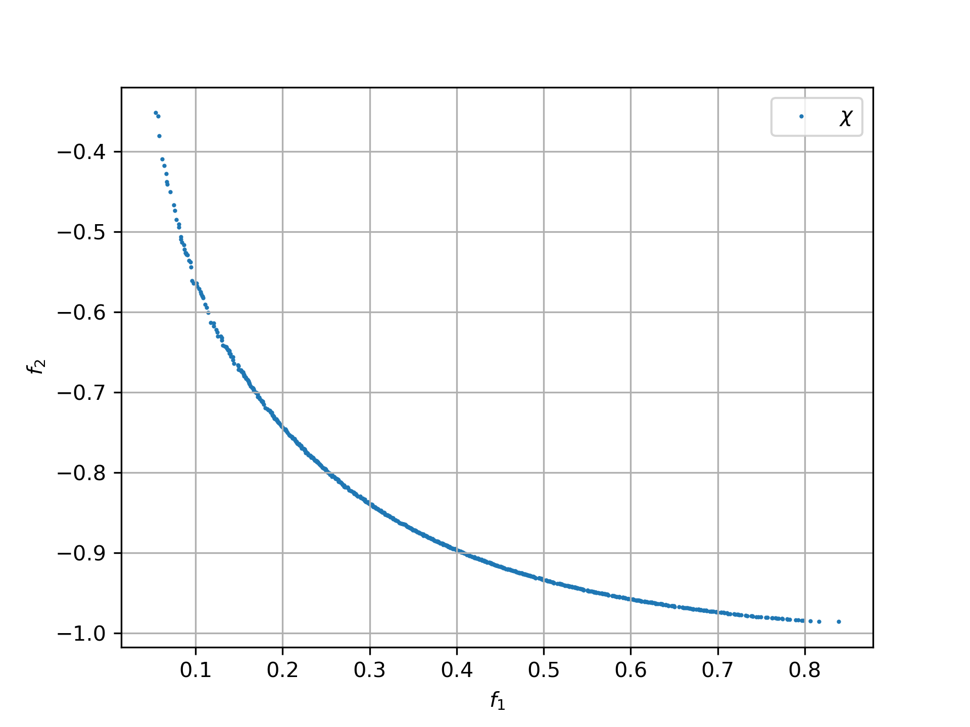
We can see that investments of 20% or 30% make sense because the ROI improvement is large. Coverage rises from 74% to 83%. For investments above 70%, the improvement in coverage is very small.
Single Objective Fitness Function
To verify the result, we also apply single-objective optimization.
We decide to invest 30%, so we use cost = max(0.3, cost) to target that cost,
and then use the weighted sum y = 2*cost + cov as a single objective.
Multi-objective optimization resulted in 83.9% coverage for 30.07 % investment:
...
0.3007221745649993, -0.8389101868937222] [1.99999, 1.16422, 0.25989, 0.18943, 0.62899, ...
...
   def fitness_so(self, x):
        cost, cov = self.cost(x)
        cost /= self.max_cost # to be minimized
        cov /= -self.max_cov # to be maximized
        cost = max(0.3, cost) # target 30% cost
        y = 2*cost + cov
        if y < self.best_y.value:
            self.best_y.value = y
            nds = nodes(x.astype(int))
            print("n,cov", cost, cov, num_true(nds), len(nds))
        return y
Single Objective Optimization
By increasing popsize and using 3000000 evaluations in each of the 32 parallel
retries, we spend much more time while focusing on a single objective.
So we expect a nearly optimal result this time.
We choose fcmaes differential evolution because, like MODE, it supports integer variables
through the ints parameter.
def opt_so(g):
    prob = problem_fb(g)
    res = retry.minimize(wrapper(prob.fitness_so),
                     prob.bounds,
                     optimizer=De_cpp(3000000, popsize = 512,
                     ints = [True]*prob.dim),
                     num_retries=32)
    print (nodes(res.x.astype(int)))
As result we see after 1315 seconds:
n,cov 0.3000079411544962 -0.8427741890749982 348 751
1315.03 92410369 70272.0 -0.24275830676600585
This means the improvement over the multi-objective optimization result (84.28% compared to 83.9% coverage at 30% investment) is quite modest. The computed pareto front, after only 217 seconds, already provided a reliable basis for the decision. We can still apply single-objective optimization afterward to squeeze out the last quarter percent.
Conclusion
-
Multi-objective optimization can provide the basis for decision making even for combinatorial problems.
-
Using anonymized Facebook data, we showed that friendship and group relationships can be analyzed with moderate computing resources to plan a targeted campaign with limited budget by selecting the most influential people in the social network.
-
Applying numba together with an efficient graph representation based on numpy arrays and a fast optimization algorithm written in C++, supporting integer decision variables and parallel retry are crucial for the success of this method.
-
fcmaes provides these algorithms for both single- and multi-objective problems.
-
After an investment decision has been made from the pareto front generated by multi-objective optimization, single-objective optimization can be used to improve the result further.