

Water Resource Management
This tutorial
-
Discusses two complex multi objective water management optimization problems.
-
Shows how the implementations can be modified to add a Python API and support Python multiprocessing to speed up objective function evaluation.
-
Shows how fcmaes-MODE and pymoo can be applied to the adapted test cases.
Motivation
Water management is important lists 10 reasons why water management matters now and will matter even more in the future. Already today, 2 billion people lack access to a safely-managed drinking water service. Most water resource challenges are multiobjective. We have to balance many competing goals when we calibrate models and plan and manage water resources. This gets even harder when the objective function includes stochastic Monte Carlo simulations.
Computed Pareto fronts for these many-objective problems can reveal important structure in the problem domain. See for instance: Visual analytics clarify the scalability and effectiveness of massively parallel many-objective optimization.
Water resource management optimization problems can be so complex that they justify the use of up to 524,288 compute cores: Evolving many-objective water management to exploit exascale computing
We do not focus on visualization here. Instead, we show how to reduce that 524,288-core requirement to a single mainstream 16-core CPU. This depends not only on the choice of optimizer, but also on speeding up objective function calls by adding a ctypes-based Python API that supports multiprocessing. The corresponding code is hosted in the following two GitHub forks, one for each problem discussed here:
Note that we are not only competing with half a million cores. The optimizer used there, Borg, is also highly sophisticated. Its source code is available for academic use, but it is still effectively a closed source product written in ANSI C and includes auto-adaptive multioperator recombination, see Borg paper.
Issues with the objective function implementations
Both implementations are efficient C++ code. Running 5000 Monte Carlo iterations takes only milliseconds. Still, the original designs create avoidable bottlenecks. The following points are worth keeping in mind for future models and problem implementations:
-
API: A command-line interface, as used for both problems, can be called from any programming language. But it can become a major performance bottleneck, especially in parallel settings. The HBV objective function can be executed 30000 times/sec on a modern 16 core CPU, so that overhead matters.
-
Implement the objective function as reentrant so multiple invocations can run safely at the same time. That also makes it much easier to add an API for another language such as Python. In practice this means: no global variables. All shared variables should be member variables of a singleton class instance. Then each reentrant API call can create its own singleton instance and avoid sharing state with parallel calls. You can inspect the two forks above to see how this was done.
-
Do not hide discrete decision variables from the optimizer. Use integer decision variables to generate the discrete values. The optimizer may use this information to adapt its algorithm, as fcmaes MODE and DE do.
-
Separate initialization code from objective function code. Sometimes initialization is expensive and should run only once.
Lower Rio Grande Valley (LRGV) problem framework
The Lower Rio Grande Valley (LRGV) problem framework implements a risk-based water supply portfolio management problem. A single city has to find an efficient mix of market-based and traditional reservoir sources for its water supply while minimizing the risk of running short of water at any time. An option-based market lets the city buy water later at a fixed price by paying an option price in advance.
The implementation https://github.com/jrkasprzyk/LRGV is highly configurable, including the choice of the objectives and the definition of the constraints.
To keep the results comparable with Visual analytics clarify the scalability and effectiveness of massively parallel many-objective optimization, we configure the problem framework to use the following five objectives:
-
minimize water supply costs
-
maximize the reliability of meeting demands
-
minimize surplus water
-
minimize dropped or unused water transfers
-
minimize the number of leases required over a 10 year planning horizon
Results
Is this problem really that hard? We reduced the number of Monte Carlo iterations from 10000 to its default 5000, which seems to be sufficient, and used a single 16 core AMD 5850x CPU for all experiments.
First we performed 8 NSGA II runs using the pymoo optimizer. Parallel function execution did not work, so we started 8 optimization runs in parallel by hand:
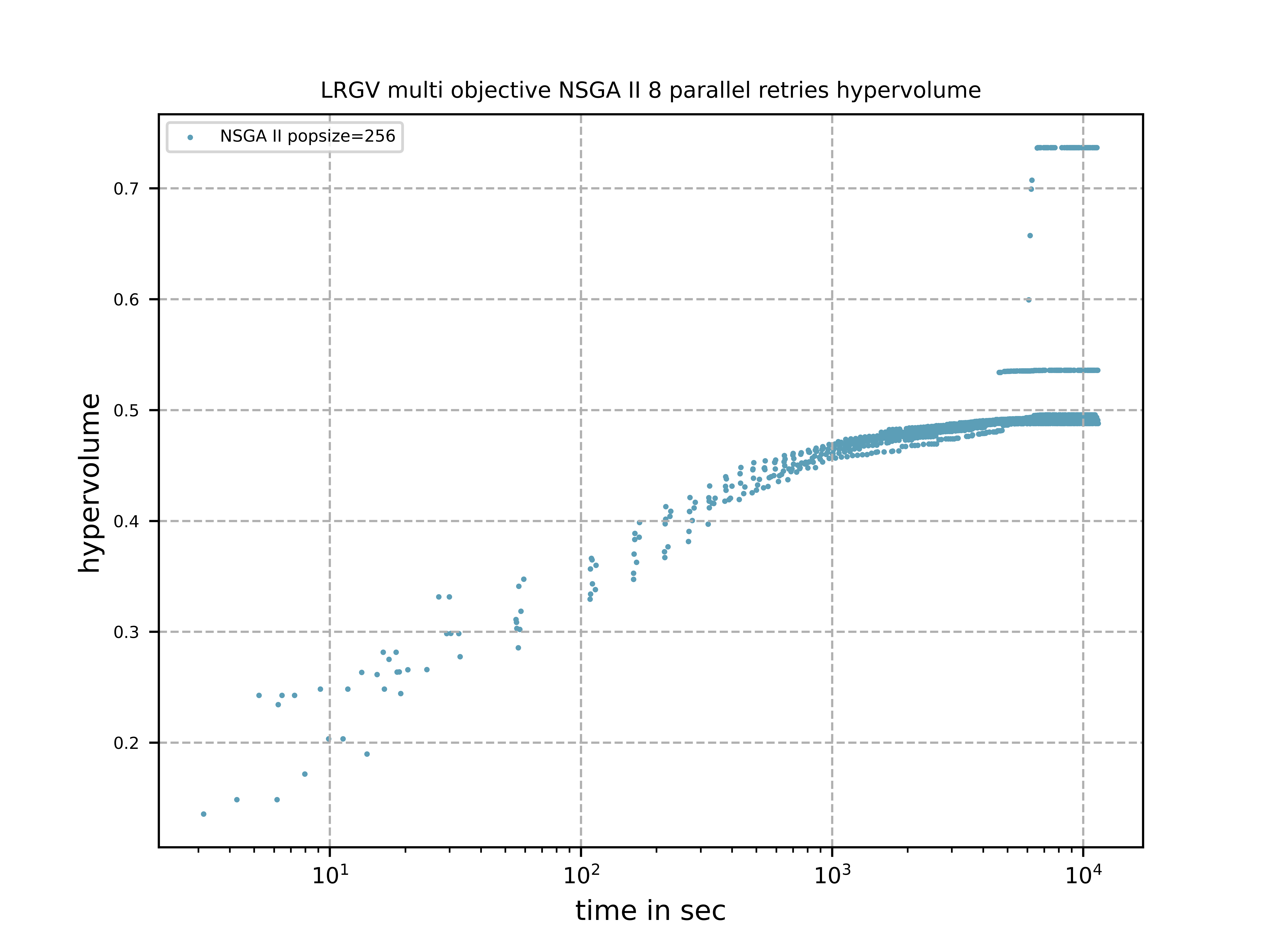
Only one of the 8 NSGA-II runs produced a reasonable result.
Then we used the fcmaes MODE with parallel function evaluation. Hypervolume normalization was done in the same way as in the previous experiment to ensure comparability.
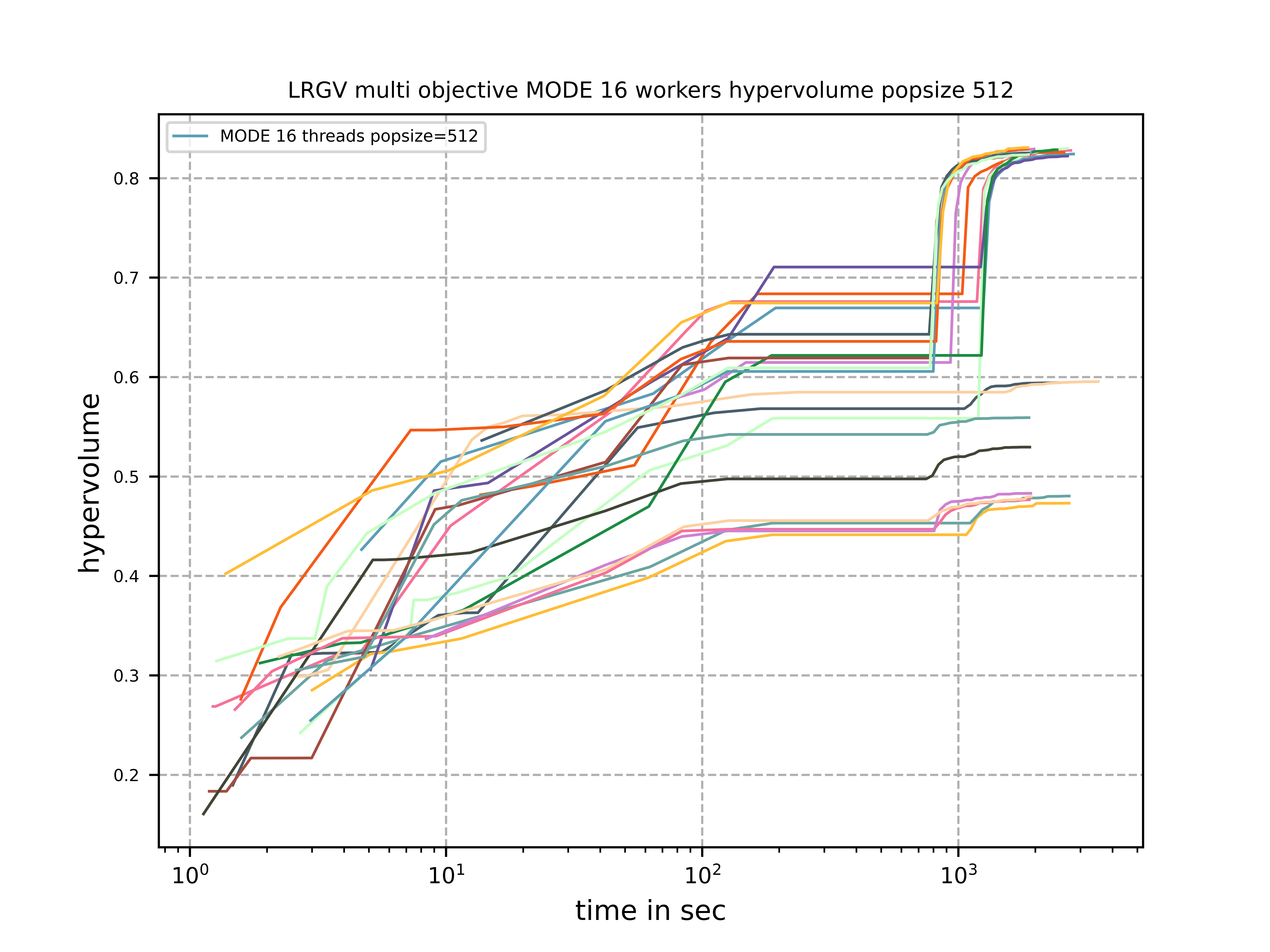
This time about half of the runs succeeded in producing a hypervolume >= 0.82. The other half got trapped in non optimal local minima.
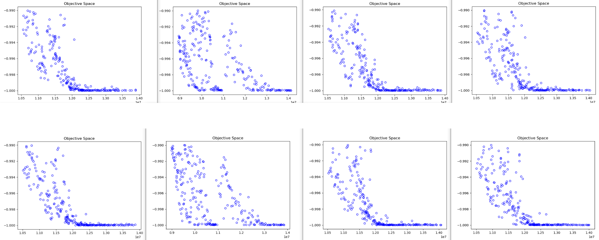
Here is a 2 dimensional projection of the 5 dimensional Pareto front showing only the first two objectives for all 8 NSGAII runs:
For comparison, here are different 2 dimensional projections of the MODE Pareto front for one of the successful runs (hypervolume > 0.82). The first one also covers the first two objectives:
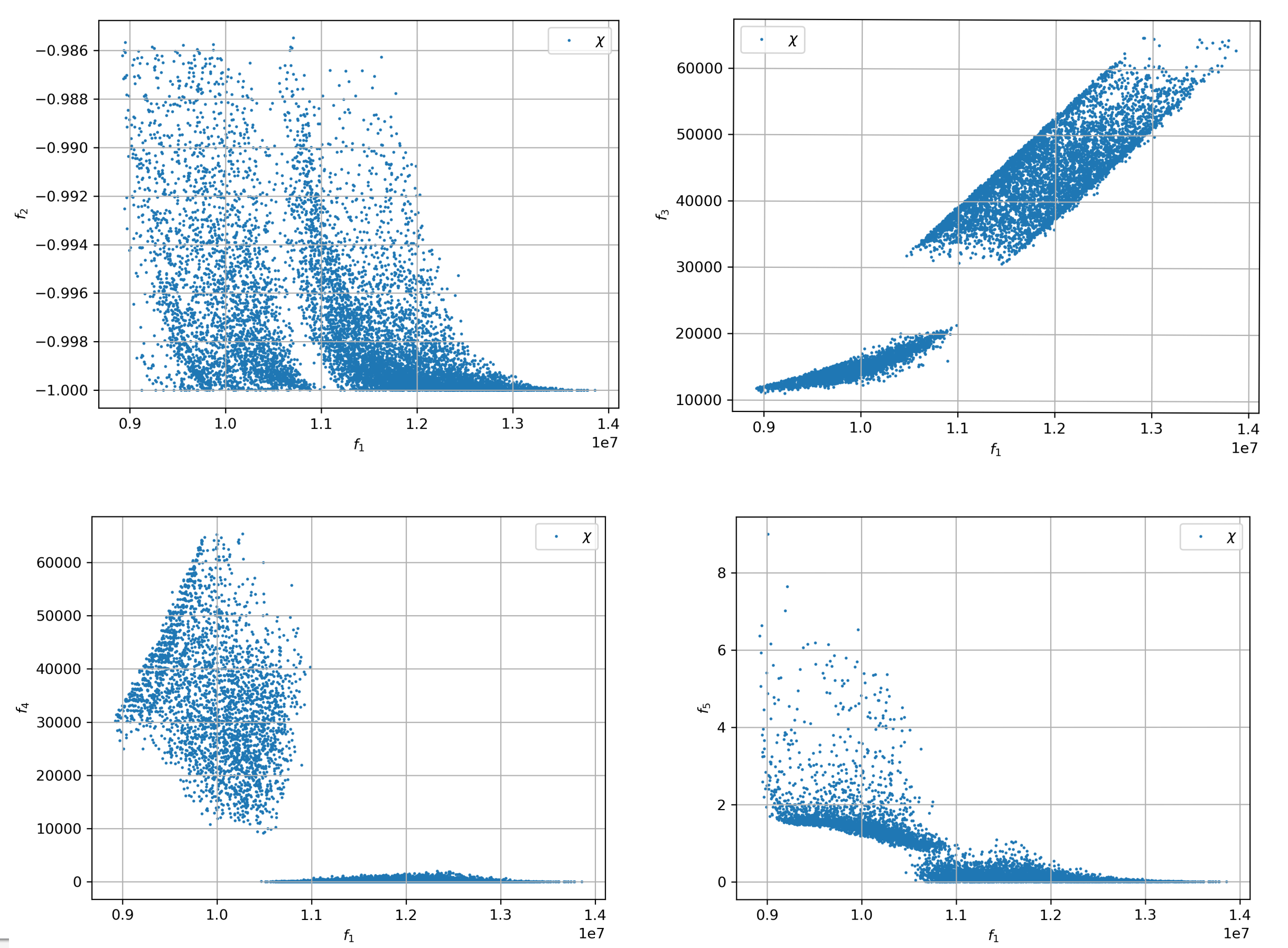
Here is the Pareto front for a failed MODE run:
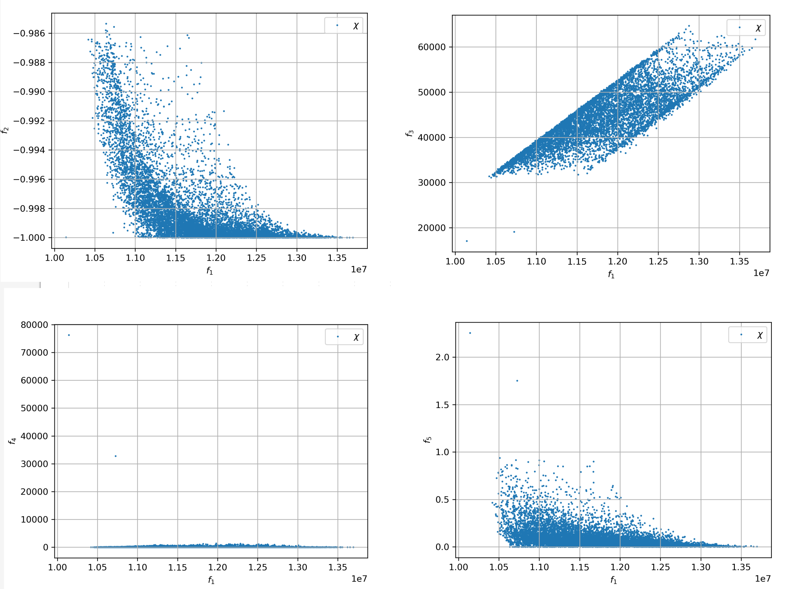
Even standard NSGA-II can produce reasonable results if you perform enough retries. But it does not do so within the 20 minute time limit used with the exascale computer, especially with 5000 instead of 10000 Monte Carlo iterations per function evaluation.
fcmaes-MODE does better. In about half of the experiments it reaches a hypervolume >= 0.82 in about 30 minutes.
Alternatively, the fcmaes MODE parallel retry mechanism can be used to perform 32 parallel MODE optimizations and merge all results into a single Pareto front. This trades additional run time for a very reliable result. Since parallel retry scales better with the number of cores, it should be preferred if time is not a concern or if you have a really big CPU >= 32 cores. If you can use a whole CPU cluster, you should use parallel function evaluation on each CPU and merge the results from all CPUs.
Unfortunately in Evolving many-objective water management to exploit exascale computing not enough details are given (what is the hypervolume scaling / the "ideal" hypervolume used) to compare the results. They report 1.2 sec per function call (10000 monte carlo iterations each), we observe about 9 evals/sec single threaded (5000 monte carlo iterations each).
MODE parallel function evaluation performs 110 evals/sec (16 threads). To fully utilize the CPU two 16 thread experiments can be executed in parallel, resulting in about 72 evals/sec each. fcmaes MODE parallel retry executes about 152 evals/sec, so it scales better than parallel function evaluation. It is not completely clear why the exascale cores are so slow.
About one hour should be sufficient for fcmaes MODE on a standard 16 core CPU to produce a very good Pareto front. Even a set of NSGA-II runs executed in parallel for two or three hours seems enough to inform decision makers about the key tradeoffs in the problem domain.
You can decide yourself if the investment in an exascale machine is justified.
How to replicate the results?
The code for this example is at lrgv.py. Adapt AllDecAll_control.txt if you want to reconfigure the experiment. But do not forget to adapt the Python code accordingly if you change the number of objectives or constraints. The shared library for linux is part of the fcmaes github repo, for other OS please use the fork at https://github.com/dietmarwo/LRGV to create one.
HBV Rainfall-Runoff Model
The rainfall-runoff multiobjective problem (see Evolutionary multiobjective optimization in water resources)
has three primary routines:
-
snow accumulation and melt
-
soil moisture accounting
-
transformation of the linear outflow from two sub-basins
The model contains 14 real-valued decision variables that require calibration. It is a "real world problem". Its corresponding multi-objective optimization problem was used to calibrate the HBV model for the Williams River in West Virginia, United States.
"If an algorithm exhibits very good performance with respect to its best single run, but only a small percentage of runs attain this good performance, it would be very difficult for users to implement effectively."
Our view is almost the opposite. Modern many-core CPUs make it possible to run many optimization runs in parallel with little extra wall-time. Diversity across individual runs can improve the overall result because we can compute the Pareto front of the combined results. A "consistent reliable" algorithm that produces the same result in every run is exactly what we do not want as the base algorithm for automated parallel retry.
As with LRGV, we forked the repository https://github.com/dietmarwo/awr-hbv-benchmark, added a Python ctypes API, and removed all global variables to enable parallel execution. This allows fcmaes MODE parallel retry to execute about 30000 evaluations per second on a single 16 core AMD 5950 CPU. As a result, HBV is not very relevant as a real-world benchmark, since it reaches nearly perfect results in a few seconds, as shown below. For this problem, unlike LRGV, parallel objective function evaluation is much slower, only about 1650 evals/sec. The reason is that function execution time is low compared to the parallelization overhead.
Here is a typical Pareto front, shown through some of its 2 dimensional projections. It looks the same for all algorithms we tried:
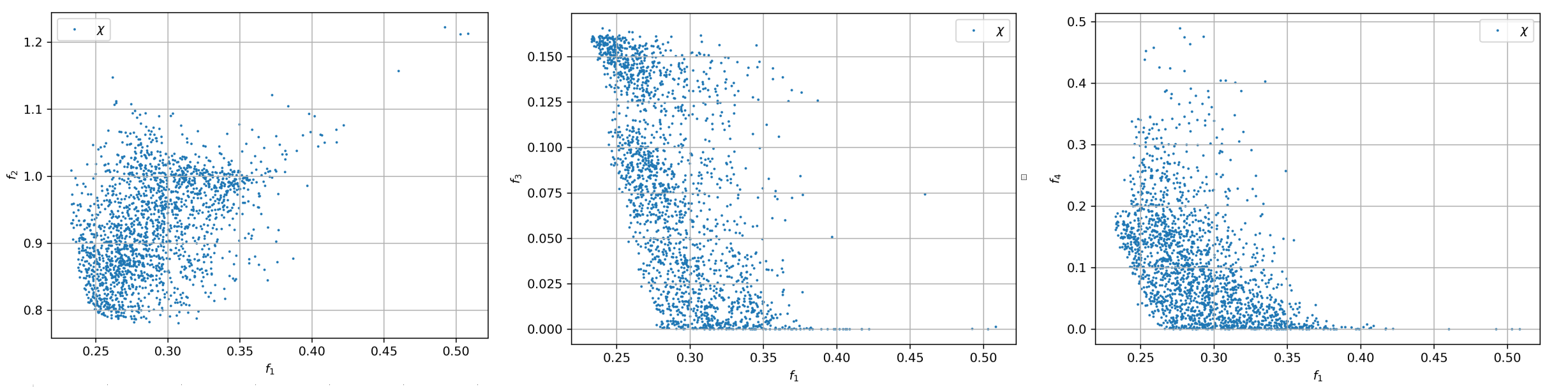
After about 100 seconds we get a nearly optimal hypervolume, independent of the algorithm used.
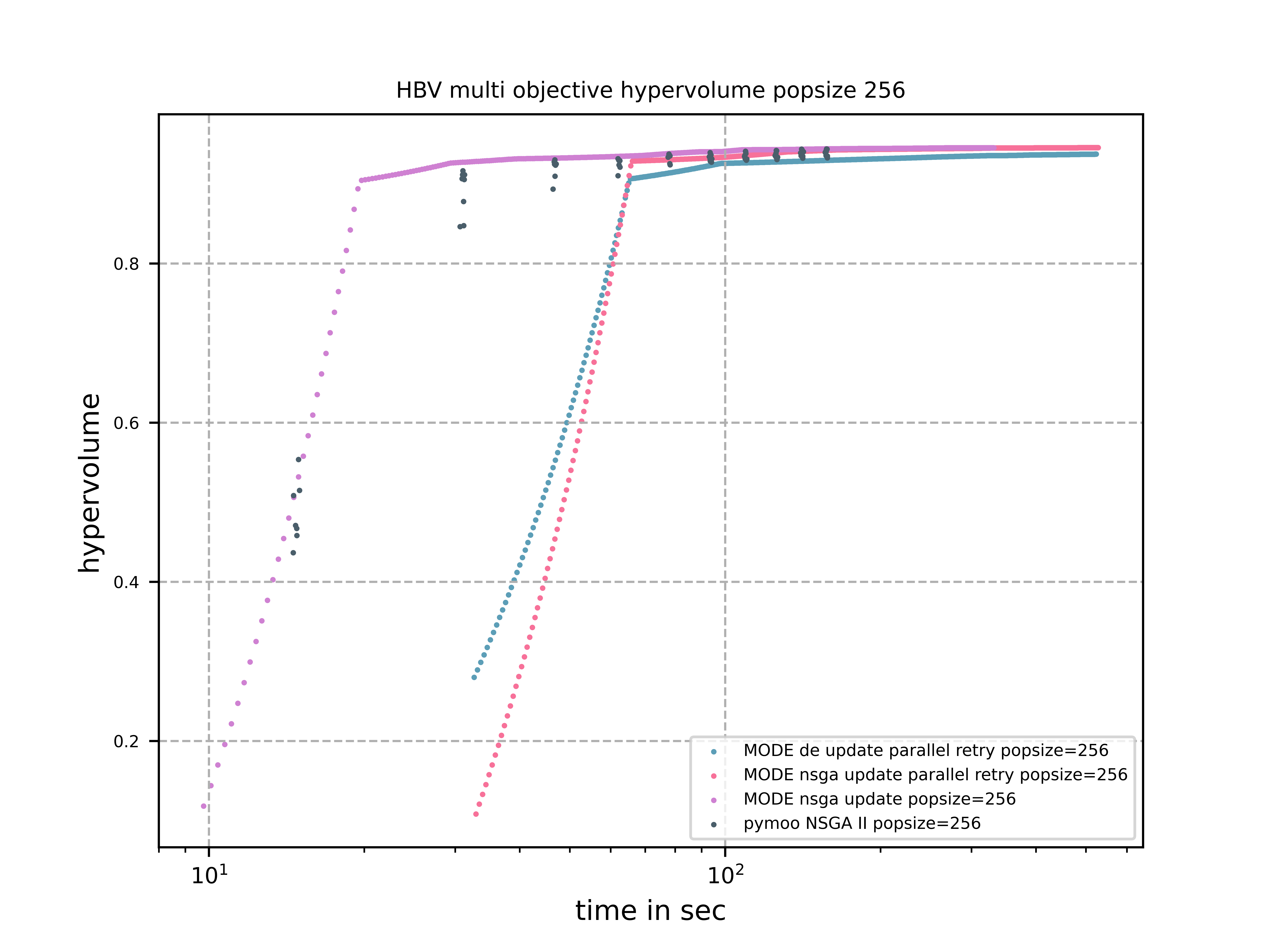
MODE using parallel function evaluation is the fastest approach here. Note that this time nsga-update=True produces better
results, which is usually not the case for more complex problems.
Even pymoo NSGA-II in a single thread works well and is very fast; applying multi-threading results in an error.
The eight pymoo NSGA-II runs differ slightly, but you can easily start multiple runs in parallel on a 16-core machine
and use the best run without any additional wall-time.
How to replicate the results?
The code for this example is at hbv.py. The shared library for linux is part of the fcmaes github repo, for other OS please use the fork at https://github.com/dietmarwo/awr-hbv-benchmark to create one.
Conclusion
We have not found a water-related multi-objective benchmark where a modern many-core CPU is not sufficient, as long as about one hour of wall time is available. Please write me if you know one. There is also a widespread misconception about algorithms whose runs produce different results, with only a small percentage reaching very good performance. In practice, these algorithms are often well suited for parallel execution. For multi-objective problems we can simply join the Pareto fronts from different parallel runs. Diversity is very helpful.