

Optimizing Crypto Trading Strategies
This tutorial shows:
-
How to retrieve and cache historical ticker data.
-
How to implement a very fast trading simulation using numba.
-
How to optimize one set of trading strategy parameters for several tickers at once.
-
How to optimize multiple objectives, one per ticker, while also handling constraints.
-
How to visualize the resulting strategy for different cryptos.
This is not a tutorial about inventing trading strategies. The goal is simpler. We take an existing strategy, turn a few parts of it into parameters, and then search for settings that fit the cryptos we want to trade.
The same idea can be used with almost any trading strategy, as long as you can implement an efficient simulation on historical data. You can optimize a single aggregated objective, or compute a Pareto front with one objective per ticker. The multi-objective view can be useful when you want to understand which parameter settings fit which subset of coins. It also works when you need extra constraints, such as an upper limit on the number of trades.
Note that this tutorial was tested on Windows, but it runs much slower there, often by more than a factor of 3. The reason is Python multi-threading on Windows. Use Linux, or the Linux subsystem on Windows, whenever possible.
Motivation
Imagine you are one of the many crypto youtubers. You probably use Tradingview and the Pine language to develop the indicators you use in your videos. Here you can find many example scripts. Tradingview also helps you test strategies on historical data. This overview compares several so-called replay simulators, including Tradingview. But even a paid premium account still has many limits.
Pine is a language built for this use case. Still, in terms of expressive power, pandas DataFrames and time series are not far behind.
The obvious advantage of using pandas is flexibility. You are no longer boxed in. You can implement strategies that:
-
Involve multiple tickers or coins.
-
Invest only part of the cash, or sell only fractions of the portfolio.
-
Consider fees and taxes.
-
Fulfill certain constraints.
-
Access external data (fundamentals)
-
…
There is also a less obvious advantage:
-
By using to_numpy(), you can convert time series into numpy arrays.
-
Those arrays can be processed with numba, which makes strategy replay very fast.
-
That speed makes standard parameter optimizers such as BiteOpt practical. The optimizer can then replay the strategy automatically while varying the parameters.
This gives you an environment where you can implement all kinds of scripts without these platform limits. You can run many thousands of replays per second, even across several coins at once. That lets you see which parameter settings fit which coin. The search can target one or many objectives, such as ROI, and it can also include constraints, such as a minimum holding time to avoid income tax.
This tutorial provides a starting point and shows how such a workflow can be built with fcmaes.
Key ideas
The main ideas behind an efficient simulation or replay are:
-
Precompute all time series data needed by the strategy and store it in a pandas data frame.
-
Use pandas
.to_numpy()to convert the relevant series into numpy arrays passed to the simulation. -
Use numba to implement the simulation on top of those arrays.
The tricky part comes from current numba limitations. In practice, numba mostly works on numpy arrays. That makes trade logging harder. We need logging not for the optimization itself, but later for plotting the buy and sell actions.
Our example strategy is intentionally simple. Even so, it already improves noticeably over HODL.
The HODL strategy used as reference point
HODL stands for "hold on for dear life" and is a well-known strategy in the crypto scene. Over longer periods, larger cryptos such as Bitcoin, Ethereum, XRP, and ADA increased strongly in the historical windows considered here, just as many stocks did.
We use a simple version of HODL as a reference: invest everything at the start of the interval and sell everything at the end. Our objective is the return on investment (ROI) of a strategy, divided by the HODL ROI for the same coin.
EMA / SMA exponential and simple moving average
The example strategy used here is very simple. Its purpose is not to recommend a real trading system. It is only meant to show how to build a fast simulation and optimization loop around a strategy.
EMA and SMA are both moving averages. The key difference is that EMA gives more weight to recent prices. We use crossings between them as buy and sell signals.
We buy when EMA crosses SMA from below. We sell when the crossing goes in the opposite direction. A short-lived crossover can quickly reverse, so we add two more parameters to slow the strategy down:
-
Minimal wait time after the last sell before buying again (
min wait buy). -
Minimal wait time after the last buy before selling again (
min wait sell).
To keep the example simple, we always invest all available cash and sell all held coins. Each simulation handles one ticker, such as Bitcoin. During optimization, however, we run the same parameters on several tickers and combine the results to reduce overfitting.
So the EMA/SMA strategy has four input parameters:
-
EMA window size.
-
SMA window size.
-
min wait buy(after the last sell). -
min wait sell(after the last buy).
Example Plot
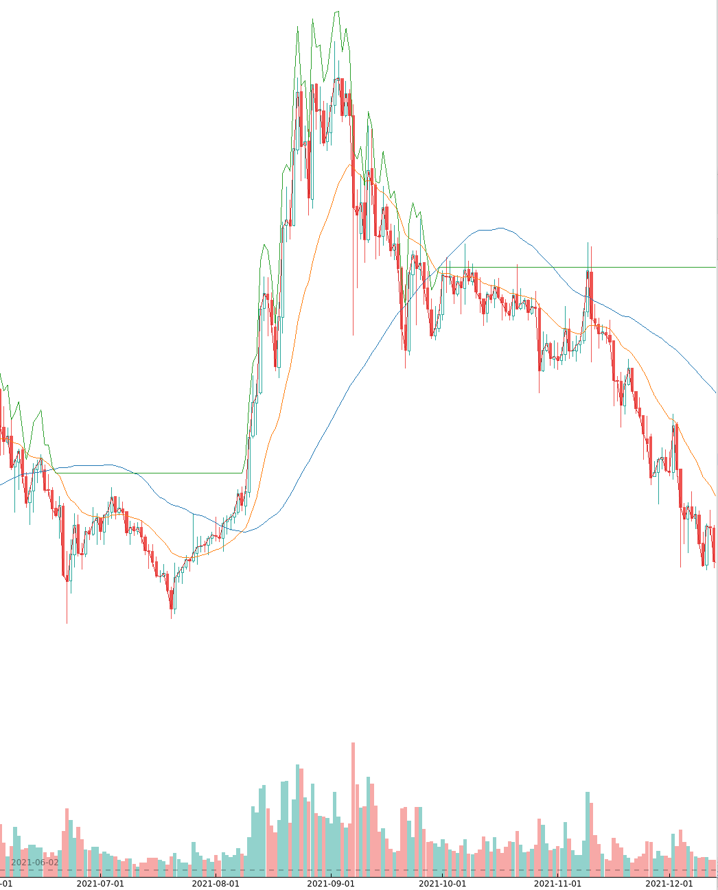
This tutorial is based on crypto.py. Adapt this code for your own experiments. The following diagram was produced with the code below:
if __name__ == '__main__':
    tickers = ['ADA-USD']
    start="2019-01-01"
    end="2030-04-30"
    fit = fitness(tickers, start, end)
fit.plot([20,60,10,10])-
The blue line represents SMA-60.
-
The orange line represents EMA-20.
-
The green line shows the value of our crypto position plus our cash.
The green line follows price changes while we are invested. It stays flat when we are holding cash. We can see the buys and sells at the crossings of the orange and blue lines. By staying in cash near the end, the strategy avoids losing money there. At the same time, it clearly does not buy at the absolute bottom or sell at the absolute top. Predicting those points exactly is hard.
fitness is the objective function used for optimization. It performs the simulation on historical
data. The same class is used both during optimization and, as here, to plot a specific parameter
setting. fit.plot([20,60,10,10]) visualizes these parameters:
-
EMA window size 20 days.
-
SMA window size 60 days.
-
min wait buy10 days after the last sell. -
min wait sell10 days after the last buy.
class fitness(object):

    def __init__(self, tickers, start, end, max_trades = None):
        self.evals = mp.RawValue(ct.c_int, 0)
        self.best_y = mp.RawValue(ct.c_double, math.inf)
        self.t0 = time.perf_counter()
        self.tickers = tickers
        self.max_trades = max_trades
        self.histories = {}
        self.closes = {}
        self.dates = {}
        self.hodls = {}
        for ticker in tickers:
            self.histories[ticker] = get_history(ticker, start=start, end=end)
            self.closes[ticker] = self.histories[ticker].Close
            self.dates[ticker] = np.array([d.strftime('%Y.%m.%d') for d in self.histories[ticker].index])
            self.hodls[ticker] = hodl(self.closes[ticker].to_numpy(), START_CASH)
For each ticker, the pandas data frame with historical data is stored in self.histories[ticker].
Everything that can be precomputed at this stage, meaning everything independent of the strategy
parameters, is stored either as numpy arrays (self.dates) or scalar values (self.hodls). EMA
and SMA depend on the parameters, so we defer their computation and keep the close prices as
pandas series in self.closes[ticker]. Values shared across process boundaries, such as the best
objective seen so far in all threads (best_y), are stored as mp.RawValue.
Caching historical ticker data
fitness first checks a local cache and downloads historical data only when needed
(get_history(ticker, start=start, end=end)). This cache is intentionally simple. If you change
either the start or end date, the whole interval is downloaded again and stored as compressed CSV
files in fast-cma-es/examples/ticker_cache.
There is no smart merging with existing data. You can choose an end date in the future to download everything available up to now, but as long as the end date stays the same, there is no further update.
Single Objective Optimization
In the single-objective case, we maximize the average strategy-ROI / HODL-ROI across several tickers. The example code uses Bitcoin, Ethereum, XRP, and ADA, but you can adapt it to any other set. Use ticker name search to look up the symbols.
    def fun(self, x):
        # simulate the EMS/SMA strategy for all tickers
        factors = []
        num_trades = []
        for ticker in self.tickers:
            # convert the optimization variables into integers and use them to configure the simulation
            f, num, _ = simulate(self.closes[ticker], int(x[0]), int(x[1]), int(x[2]), int(x[3]))
            factors.append(f)
            num_trades.append(num)
        factor = np.prod(factors) ** (1.0/len(factors)) # normalize the accumulated factor
        y = -factor # our optimization algorithm minimizes the resulting value, we maximize factor
fun is used both by the single-objective case (call(self, x)) and the multi-objective
case (mofun(self, x)). It computes the geometric mean of the f = strategy-ROI / HODL-ROI
values, which we want to maximize.
def simulate(prices, ema_period, sma_period, wait_buy, wait_sell, dates=None):
    close = prices.to_numpy()
    ema = get_ema(prices, ema_period)
    sma = get_sma(prices, sma_period)
    return strategy(close, START_CASH, ema, sma, wait_buy, wait_sell, dates)
simulate uses pandas built-in functions to compute EMA and SMA from the parameters, then calls
strategy, which is annotated with @njit. That means numba compiles
the time-critical part of the replay. Keeping the Python interpreter out of this inner loop is
essential for performance.
Because of numba limitations, strategy cannot handle logging in a convenient way. Instead, it
can optionally collect the trading history, meaning the buy and sell actions, in a list of
strings called logs. The objective function does not need this. We use it later when plotting
a strategy.
Let’s try it. Adapt and run crypto.py like this:
if __name__ == '__main__':
    tickers = ['BTC-USD', 'ETH-USD', 'XRP-USD', 'ADA-USD']
    start="2019-01-01"
    end="2030-04-30"
    fit = fitness(tickers, start, end)
    optimize(tickers, start, end)
This produces output like:
hodl = 10.976 [11.4, 22.1, 2.3, 25.5]
nsim = 1: time = 1.1 fac = 0.273 [0.5, 0.1, 0.3, 0.3] ntr = [8, 8, 8, 6] x = [40, 86, 137, 90]
nsim = 7: time = 1.1 fac = 0.304 [1.3, 0.3, 0.3, 0.1] ntr = [8, 10, 10, 10] x = [47, 90, 68, 102]
nsim = 21: time = 1.1 fac = 0.401 [0.2, 0.3, 0.8, 0.4] ntr = [5, 4, 4, 4] x = [43, 74, 195, 145]
nsim = 22: time = 1.1 fac = 0.937 [1.6, 0.6, 1.1, 0.7] ntr = [8, 10, 10, 11] x = [48, 59, 35, 168]
nsim = 104: time = 1.2 fac = 1.119 [1.8, 0.7, 0.6, 2.1] ntr = [10, 10, 12, 10] x = [37, 63, 44, 95]
nsim = 245: time = 1.2 fac = 1.236 [1.1, 0.9, 1.8, 1.2] ntr = [10, 10, 10, 10] x = [39, 62, 12, 138]
nsim = 317: time = 1.2 fac = 1.566 [2.5, 0.3, 2.7, 2.6] ntr = [10, 12, 10, 10] x = [40, 60, 24, 113]
nsim = 377: time = 1.2 fac = 2.031 [1.7, 0.9, 3.4, 3.2] ntr = [10, 10, 10, 10] x = [21, 56, 18, 109]
nsim = 938: time = 1.2 fac = 2.145 [2.1, 1.1, 3.2, 3.0] ntr = [10, 10, 10, 10] x = [27, 57, 28, 104]
nsim = 8053: time = 1.5 fac = 2.220 [2.1, 1.2, 3.2, 3.0] ntr = [10, 10, 10, 10] x = [26, 57, 17, 104]
nsim = 14210: time = 1.8 fac = 2.243 [2.1, 1.1, 3.5, 3.3] ntr = [10, 10, 12, 10] x = [27, 57, 22, 98]
nsim = 15697: time = 1.9 fac = 2.261 [2.1, 1.1, 3.6, 3.3] ntr = [10, 10, 12, 10] x = [27, 57, 24, 98]
nsim = 23261: time = 2.1 fac = 2.273 [2.1, 1.1, 3.6, 3.3] ntr = [10, 10, 12, 10] x = [26, 57, 23, 98]
nsim = 29273: time = 2.4 fac = 2.282 [2.1, 1.1, 3.5, 3.3] ntr = [10, 10, 12, 10] x = [26, 57, 25, 97]
nsim = 34236: time = 2.6 fac = 2.283 [2.1, 1.1, 3.6, 3.3] ntr = [10, 10, 12, 10] x = [26, 57, 24, 98]
hodl = 10.976 means that the HODL strategy would have grown the initial investment by about a
factor of 11 from 2019 until now. That helps explain both the interest in crypto and the
popularity of HODL.
After 34236 simulations in about 2.6 seconds, the optimizer ends at x = [26, 57, 24, 98]. That
means EMA-26, SMA-57, a minimum wait of 24 days before buying, and a minimum wait of 98 days
before selling, even when the signal says otherwise. This parameter set works well for BTC, XRP,
and ADA, but much less well for ETH, where the factor is only 1.1.
The run rate is more than 10000 simulations per second on an AMD 5950x 16-core CPU using 32 parallel threads. That leaves plenty of room for more complex and more expensive strategies. Even if an optimization took 2 hours instead of 2 seconds, that could still be acceptable in practice.
How to fight FOMO
How much did we earn on average with the optimized parameters? Multiply the HODL factor by
2.283, the final single-objective value. 2.283 * 10.976 = 25, so in this backtest we would
have ended up about 25 times richer over roughly three years. Results like that explain why
FOMO is such a big topic in crypto.
If you want an antidote to FOMO, you can always read one of the 400 Bitcoin obituaries predicting that Bitcoin will soon be worthless. Another option is to change the start and end dates and optimize over a bear-market window instead. In practice, FOMO and its counterpart FUD (Fear, Uncertainty, and Doubt) are useful to us. Emotion-driven trading is exactly the kind of behavior a strategy tries to exploit.
We did not account for fees or taxes here. That is left as an exercise.
Which trades were performed?
Another part of the output lists the actual trades performed by the optimized strategy:
BTC-USD

2019.02.25 cash 1000000 buy 257 num_coins 0 price 388269 ct
2019.08.02 cash 2147 sell 257 num_coins 257 price 1051817 ct
2019.11.06 cash 2705317 buy 289 num_coins 0 price 936087 ct
2020.03.06 cash 23 sell 289 num_coins 289 price 912254 ct
2020.04.24 cash 2636439 buy 349 num_coins 0 price 755090 ct
2020.09.10 cash 1175 sell 349 num_coins 349 price 1036313 ct
2020.10.14 cash 3617910 buy 316 num_coins 0 price 1142950 ct
2021.04.26 cash 6186 sell 316 num_coins 316 price 5402175 ct
2021.07.29 cash 17077060 buy 426 num_coins 0 price 4000842 ct
2021.11.27 cash 33472 sell 426 num_coins 426 price 5481507 ct
2022.02.14 cash 23384696 sell 0 num_coins 0 price 4260470 ct

ETH-USD

2019.02.25 cash 1000000 buy 7151 num_coins 0 price 13982 ct
2019.07.17 cash 126 sell 7151 num_coins 7151 price 21148 ct
2019.09.23 cash 1512455 buy 7490 num_coins 0 price 20192 ct
2019.12.31 cash 65 sell 7490 num_coins 7490 price 12961 ct
2020.01.25 cash 970850 buy 6019 num_coins 0 price 16128 ct
2020.09.17 cash 82 sell 6019 num_coins 6019 price 38901 ct
2020.10.22 cash 2341589 buy 5659 num_coins 0 price 41377 ct
2021.06.03 cash 47 sell 5659 num_coins 5659 price 285512 ct
2021.08.01 cash 16157208 buy 6306 num_coins 0 price 256185 ct
2021.12.10 cash 2169 sell 6306 num_coins 6306 price 390849 ct
2022.02.14 cash 24649145 sell 0 num_coins 0 price 294495 ct

XRP-USD

2019.03.07 cash 1000000 buy 3176963 num_coins 0 price 31 ct
2019.07.08 cash 0 sell 3176963 num_coins 3176963 price 40 ct
2019.10.12 cash 1275655 buy 4669464 num_coins 0 price 27 ct
2020.03.07 cash 0 sell 4669464 num_coins 4669464 price 23 ct
2020.04.24 cash 1106994 buy 5716027 num_coins 0 price 19 ct
2020.09.11 cash 0 sell 5716027 num_coins 5716027 price 24 ct
2020.10.24 cash 1390663 buy 5423149 num_coins 0 price 25 ct
2021.01.31 cash 0 sell 5423149 num_coins 5423149 price 49 ct
2021.02.25 cash 2669892 buy 6144407 num_coins 0 price 43 ct
2021.06.04 cash 0 sell 6144407 num_coins 6144407 price 97 ct
2021.08.06 cash 5961279 buy 7985499 num_coins 0 price 74 ct
2021.11.25 cash 0 sell 7985499 num_coins 7985499 price 103 ct
2022.02.14 cash 8240141 sell 0 num_coins 0 price 79 ct

ADA-USD

2019.02.25 cash 1000000 buy 22705083 num_coins 0 price 4 ct
2019.07.06 cash 0 sell 22705083 num_coins 22705083 price 7 ct
2019.11.10 cash 1755897 buy 39944892 num_coins 0 price 4 ct
2020.03.08 cash 0 sell 39944892 num_coins 39944892 price 4 ct
2020.04.24 cash 1729254 buy 41302527 num_coins 0 price 4 ct
2020.08.27 cash 0 sell 41302527 num_coins 41302527 price 10 ct
2020.10.17 cash 4412101 buy 41582798 num_coins 0 price 10 ct
2021.06.18 cash 0 sell 41582798 num_coins 41582798 price 141 ct
2021.08.08 cash 58856124 buy 41220681 num_coins 0 price 142 ct
2021.11.15 cash 0 sell 41220681 num_coins 41220681 price 201 ct
2022.02.14 cash 83083873 sell 0 num_coins 0 price 104 ct
And finally we get four plots, one for each ticker:
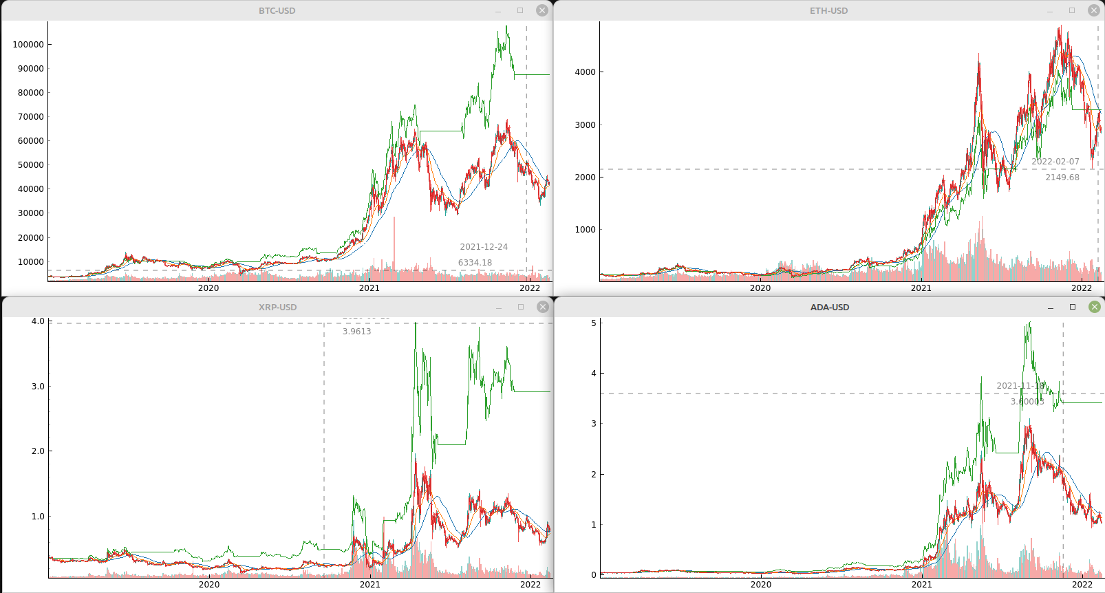
These plots again show that Ethereum is the weakest fit for this parameter set. This is the code that runs the optimization and generates the plots:
def optimize(tickers, start, end):
    bounds = Bounds([20,50,10,10], [50,100,200,200])
    fit = fitness(tickers, start, end)
    ret = retry.minimize(fit, bounds, logger = None, num_retries=32, optimizer=Bite_cpp(2000))
    fit.plot(ret.x)
We define lower and upper bounds for each strategy parameter. Different bounds can lead to
different solutions. The optimizer used here, Bite_cpp(2000)
(BiteOpt by Aleksey Vaneev, configured to run 2000
simulations per parallel retry), can be replaced. fcmaes offers many alternatives. Still,
optimizer choice is not the main point of this tutorial. BiteOpt works very well for this crypto
example.
Tax in Germany
Now imagine a friend from Germany calls and says: "That doesn’t work for me. I have to pay a huge amount of income tax if I sell after less than one year." There are two ways to handle this:
a) Change the simulation so it subtracts tax from the account when we sell before one year. Then the optimizer can decide whether selling early is still worth it.
b) Change the bounds so they enforce the rule that we always sell only after at least one year.
We will show the second option. The bounds then become:
def optimize(tickers, start, end):
    # changed so so we wait at least 365 days until we sell
    bounds = Bounds([20,50,10,365], [50,100,200,800])
    fit = fitness(tickers, start, end)
    ret = retry.minimize(fit, bounds, logger = None, num_retries=32, optimizer=Bite_cpp(2000))
    fit.plot(ret.x)
As expected, this produces fewer trades, and the optimal factor drops. 1.989 * 10.976 is still
around factor 22, so we would not lose much even if we want to avoid paying income tax.
hodl = 11.305 [11.7, 23.1, 2.3, 26.2]
nsim = 1: time = 1.5 fac = 0.763 [1.3, 0.8, 0.5, 0.6] ntr = [3, 3, 3, 3] x = [41, 69, 15, 673]
nsim = 3: time = 1.5 fac = 1.032 [1.3, 1.0, 1.4, 0.6] ntr = [3, 3, 3, 3] x = [40, 63, 11, 777]
nsim = 22: time = 1.6 fac = 1.162 [1.4, 1.0, 1.5, 0.9] ntr = [3, 3, 3, 3] x = [34, 58, 15, 795]
nsim = 63: time = 1.6 fac = 1.175 [1.3, 1.0, 1.6, 0.9] ntr = [3, 3, 3, 3] x = [43, 61, 17, 794]
nsim = 71: time = 1.6 fac = 1.215 [1.4, 1.0, 1.6, 1.0] ntr = [3, 3, 3, 3] x = [38, 56, 41, 797]
nsim = 278: time = 1.9 fac = 1.228 [1.5, 0.9, 2.1, 0.8] ntr = [3, 3, 3, 3] x = [49, 53, 11, 788]
nsim = 283: time = 1.9 fac = 1.587 [1.7, 1.2, 3.1, 1.0] ntr = [5, 5, 5, 5] x = [49, 50, 56, 372]
nsim = 2022: time = 2.2 fac = 1.634 [1.9, 1.3, 2.9, 0.9] ntr = [5, 5, 5, 5] x = [49, 50, 42, 371]
nsim = 2428: time = 2.3 fac = 1.808 [1.9, 1.3, 3.7, 1.1] ntr = [5, 5, 5, 5] x = [49, 51, 17, 369]
nsim = 2536: time = 2.3 fac = 1.858 [2.2, 1.4, 3.2, 1.2] ntr = [5, 5, 5, 5] x = [48, 50, 15, 365]
nsim = 4327: time = 2.6 fac = 1.861 [1.9, 1.3, 3.7, 1.3] ntr = [5, 5, 5, 5] x = [49, 51, 30, 371]
nsim = 6187: time = 2.8 fac = 1.892 [2.2, 1.3, 3.7, 1.2] ntr = [5, 5, 5, 5] x = [49, 51, 17, 365]
nsim = 10653: time = 3.2 fac = 1.910 [2.1, 1.3, 3.7, 1.3] ntr = [5, 5, 5, 5] x = [49, 51, 31, 366]
nsim = 11384: time = 3.3 fac = 1.940 [2.2, 1.3, 3.7, 1.3] ntr = [5, 5, 5, 5] x = [49, 51, 35, 365]
nsim = 21731: time = 4.0 fac = 1.989 [2.2, 1.3, 3.7, 1.5] ntr = [5, 5, 5, 5] x = [49, 51, 36, 365]

BTC-USD

2019.02.21 cash 1000000 buy 252 num_coins 0 price 395411 ct
2020.02.28 cash 3562 sell 252 num_coins 252 price 867245 ct
2020.04.14 cash 2189020 buy 319 num_coins 0 price 684242 ct
2021.04.15 cash 6286 sell 319 num_coins 319 price 6331401 ct
2021.06.28 cash 20203456 buy 586 num_coins 0 price 3443433 ct
2022.02.16 cash 24935 sell 586 num_coins 586 price 4372128 ct

ETH-USD

2019.02.21 cash 1000000 buy 6843 num_coins 0 price 14613 ct
2020.03.10 cash 26 sell 6843 num_coins 6843 price 20076 ct
2020.04.17 cash 1373876 buy 8004 num_coins 0 price 17163 ct
2021.05.27 cash 81 sell 8004 num_coins 8004 price 273648 ct
2021.07.25 cash 21902935 buy 9995 num_coins 0 price 219137 ct
2022.02.16 cash 154 sell 9995 num_coins 9995 price 307714 ct

XRP-USD

2019.02.24 cash 1000000 buy 3317376 num_coins 0 price 30 ct
2020.03.02 cash 0 sell 3317376 num_coins 3317376 price 23 ct
2020.04.13 cash 792013 buy 4218853 num_coins 0 price 18 ct
2021.05.17 cash 0 sell 4218853 num_coins 4218853 price 149 ct
2021.07.23 cash 6312669 buy 10361820 num_coins 0 price 60 ct
2022.02.16 cash 0 sell 10361820 num_coins 10361820 price 81 ct

ADA-USD

2019.02.27 cash 1000000 buy 23110700 num_coins 0 price 4 ct
2020.03.01 cash 0 sell 23110700 num_coins 23110700 price 4 ct
2020.04.15 cash 1061520 buy 33315151 num_coins 0 price 3 ct
2021.04.16 cash 0 sell 33315151 num_coins 33315151 price 141 ct
2021.05.23 cash 47205871 buy 35615353 num_coins 0 price 132 ct
2022.02.16 cash 0 sell 35615353 num_coins 35615353 price 107 ct
Here are the new plots:
Multi Objective Optimization
For multi-objective optimization, we compute a Pareto front, a set of non-redundant and non-dominated solutions. Each ticker gets its own strategy-ROI / HODL-ROI objective. In addition, we add simple example constraints: a maximum number of trades for each ticker.
Why use a multi-objective algorithm instead of a weighted sum?
-
The scale of the objectives does not matter. We could optimize the raw strategy ROI directly, without normalizing by HODL ROI.
-
Constraints are prioritized only while they are violated. Once they are satisfied, their scaling no longer matters either.
The tradeoff is that we usually need more simulations. Without numba, this would be much harder to do efficiently.
Looking at the Pareto front also shows whether one coin is incompatible with the others for a given strategy family. If that happens, we can optimize it separately, with the usual risk of overfitting, or remove it from the set.
    def mofun(self, x):
        _, factors, num_trades = self.fun(x)
        ys = [-f for f in factors] # higher factor is better
        constraints = [ntr - self.max_trades for ntr in num_trades] # at most max_trades trades
        return np.array(ys + constraints)
The multi-objective fitness function concatenates the objectives [-f for f in factors] and the
constraints [ntr - self.max_trades for ntr in num_trades], then returns the combined array.
-
Why do we change the sign of the objectives? The optimizer minimizes both objectives and constraints > 0, so we flip the sign to maximize profit.
-
How does the optimizer know which entries are objectives and which are constraints? The number of objectives is passed as a configuration parameter, and the optimizer assumes the objectives come first.
-
What does the optimizer do differently with constraints? Constraints are prioritized while they are violated (
c > 0). Oncec ⇐ 0, they are ignored by the optimization process. -
Is the scaling of objectives or constraints relevant? No. The optimizer treats all objectives equally, independent of scaling.
-
What about equality constraints
(a = b)? Encode them asc = abs(a-b). Then the optimizer will try to makeaandbequal. If small deviations are acceptable, usec = abs(a-b) - eps. -
What if you want to parameterize the order of a sequence of trading activities? Use input parameters in the
[0,1]interval and applynumpy.argsortto get a sequence of integers representing the order. See noisy TSP for an example.
These answers summarize why a multi-objective optimizer often makes more sense here than a
weighted-sum approach with a single-objective optimizer. Parallel retry with varying weights, as
supported by fcmaes, can partly compensate for the limitations of weighted sums.
def optimize_mo(tickers, start, end, nsga_update = True):
    nobj = len(tickers) # number of objectives
    ncon = nobj # number of constraints
    max_trades = 8
    fit = fitness(tickers, start, end, max_trades)
    bounds = Bounds([20,50,10,10], [50,100,200,200])
    xs, front = modecpp.retry(fit.mofun, len(tickers), ncon, bounds, num_retries=32, popsize = 48, max_evaluations = 16000, nsga_update = nsga_update, logger = logger())
This shows how to call the modecpp optimizer. Instead of one run, we launch as many parallel
retries as the processor can support. After that, the Pareto front for all retries is returned as
xs, front. xs contains the strategy parameters, and front contains the corresponding
objective and constraint values for the configured trading strategy.
Unlike the single-objective case, fcmaes does not offer another C++-based multi-objective
optimizer besides modecpp,
apart from its Python implementation mode.py.
Multi-objective optimization is still less established than single-objective optimization. You can
at least choose the population update mechanism with nsga_update. That lets you switch between
NSGA-II and a differential-evolution style update. If you do not care about the difference, the
default nsga_update = True is fine for this crypto example.
Let’s try it. Adapt and run crypto.py like this:
if __name__ == '__main__':
    tickers = ['BTC-USD', 'ETH-USD', 'XRP-USD', 'ADA-USD']
    start="2019-01-01"
    end="2030-04-30"
    fit = fitness(tickers, start, end)
    optimize_mo(tickers, start, end)
This gives:
nsim = 1: time = 1.1 fac = 0.412 [0.6, 0.2, 0.7, 0.3] ntr = [8, 8, 8, 6] x = [22, 77, 126, 100]
nsim = 5: time = 1.1 fac = 0.458 [1.0, 0.4, 0.5, 0.2] ntr = [8, 8, 8, 7] x = [24, 60, 97, 155]
nsim = 6: time = 1.1 fac = 0.514 [0.8, 0.4, 0.6, 0.4] ntr = [10, 10, 10, 10] x = [26, 53, 78, 118]
nsim = 9: time = 1.1 fac = 0.632 [0.9, 0.8, 0.4, 0.6] ntr = [8, 8, 9, 7] x = [25, 70, 38, 187]
nsim = 10: time = 1.1 fac = 0.719 [1.2, 0.5, 0.6, 0.8] ntr = [8, 8, 8, 8] x = [47, 66, 70, 172]
nsim = 17: time = 1.1 fac = 0.913 [1.1, 0.9, 1.1, 0.6] ntr = [8, 10, 10, 10] x = [20, 72, 32, 141]
nsim = 31: time = 1.1 fac = 1.259 [1.3, 1.6, 1.7, 0.7] ntr = [10, 8, 10, 10] x = [30, 63, 26, 139]
nsim = 122: time = 1.1 fac = 1.304 [1.4, 0.3, 2.0, 3.9] ntr = [10, 14, 12, 10] x = [24, 54, 19, 91]
nsim = 304: time = 1.2 fac = 2.006 [2.0, 1.0, 3.2, 2.5] ntr = [10, 10, 10, 10] x = [23, 58, 21, 110]
nsim = 564: time = 1.2 fac = 2.024 [1.8, 0.9, 3.4, 3.1] ntr = [10, 10, 10, 10] x = [22, 57, 14, 104]
nsim = 2801: time = 1.3 fac = 2.054 [1.8, 0.9, 3.4, 3.2] ntr = [10, 10, 10, 10] x = [23, 57, 14, 103]
The best factor reported here, fac = 2.054, is lower than in the single-objective run because
we added constraints. Those constraints are actually violated in this progress line:
ntr = [10, 10, 10, 10] exceeds the limit of 8. The reason is that this progress output tracks
only the aggregate "single-objective" view, not constraint satisfaction. After that, we get a
dump of the full Pareto front:
fac [2.68, 0.53, 0.61, 0.52] trades [8, 8, 8, 8] x = [50, 50, 89, 147]
fac [2.67, 0.73, 1.42, 0.24] trades [8, 8, 8, 8] x = [45, 51, 114, 104]
fac [2.67, 0.75, 0.92, 0.32] trades [8, 8, 8, 8] x = [45, 51, 114, 103]
fac [2.66, 0.53, 0.83, 1.08] trades [8, 8, 8, 8] x = [49, 56, 77, 171]
fac [2.65, 0.69, 1.53, 0.23] trades [8, 8, 8, 8] x = [45, 51, 114, 105]
...
fac [1.93, 0.81, 1.66, 1.35] trades [8, 8, 8, 8] x = [47, 50, 72, 184]
fac [1.93, 0.74, 1.91, 1.22] trades [8, 8, 8, 8] x = [46, 50, 75, 182]
fac [1.93, 0.77, 1.85, 1.5] trades [8, 8, 8, 8] x = [46, 50, 71, 185]
fac [1.92, 0.89, 2.53, 0.82] trades [8, 8, 8, 8] x = [50, 50, 66, 189]
...
fac [1.42, 0.33, 2.21, 1.55] trades [8, 8, 8, 8] x = [49, 51, 62, 190]
fac [1.42, 1.21, 2.01, 1.48] trades [8, 8, 8, 7] x = [49, 52, 60, 199]
fac [1.42, 1.02, 2.47, 1.4] trades [8, 8, 8, 7] x = [47, 50, 58, 199]
fac [1.41, 1.12, 2.59, 1.23] trades [8, 8, 8, 7] x = [50, 50, 43, 200]
...
fac [0.4, 1.37, 3.59, 1.55] trades [9, 10, 11, 11] x = [49, 51, 41, 163]
fac [0.31, 0.26, 0.29, 0.57] trades [7, 7, 7, 5] x = [50, 51, 88, 199]
fac [0.26, 0.14, 0.48, 0.33] trades [7, 7, 7, 7] x = [45, 50, 113, 185]
fac [0.15, 0.16, 1.31, 0.57] trades [7, 7, 7, 6] x = [50, 50, 105, 183]
Most of these solutions satisfy the constraint. We could filter out the ones that do not.