fcmaes - a Python 3 gradient-free optimization library

Determine Robust Routes for the Noisy Traveling Salesman Problem

This tutorial

shows how to implement the noisy TSP efficiently with numba when the goal is a robust route,
compares this with an alternative implementation,
compares different optimization algorithms on both implementations,
uses optimization to evaluate machine-learning-based results for another TSP variant.

The performance differences are dramatic. Depending on the optimizer and the objective-function implementation, the gap can exceed a factor of 10000. The tutorial is meant to sharpen your instincts for this kind of problem. In Python, both the objective-function design and the optimizer choice matter a lot. They affect not only evaluations per second, but also how many evaluations the same optimizer needs.

As a starting point we use TSP.py from the ExpensiveOptimBenchmark suite of the Technical University of Delft. In Hospital we discuss four other problems from the same suite. For this TSP problem, however, we also provide our own alternative implementation.

All results were produced on a 16-core / 32-thread AMD CPU 5950x. Some algorithms use only a single thread. Others use the whole processor.

Motivation

From Black-box Combinatorial Optimization using Models with Integer-valued Minima:

"When a black-box optimization objective can only be evaluated with costly or noisy measurements, most standard optimization algorithms are unsuited to find the optimal solution. Specialized algorithms that deal with exactly this situation make use of surrogate models."

The paper presents such a method, specialized for integer-valued minima: (IDONE). It is applied to a noisy variant of an asymmetric traveling salesman problem with 17 cities.

The claim that "most standard optimization algorithms are unsuited" is probably fair. But that still leaves an important question: which standard algorithms are suited? Here we identify standard algorithms that work well on TSP.py, the objective-function implementation used in the paper. We also show that an alternative implementation of the same noisy TSP problem (100 iterations, noise=1.0), noisy_tsp.py, can solve the noisy 17-city problem BR17 in about 2 seconds by using the parallel threads of modern CPUs.

The paper also studies another problem. That one is artificial and is based on matrix multiplication with random matrices and the objective function

f(x) = (x − x^∗ )^T A(x − x^∗)

for binary input values. There IDONE does use far fewer function evaluations than all standard algorithms we tried. But what happens if we change the dimension from 100 to 5000? IDONE does not scale well in that setting. I was not able to apply it successfully. A standard algorithm, BiteOpt, needs about 900.000 function evaluations and about 5 hours on a single thread, but it does solve the problem. One possible objection is that real-world problems are too expensive to evaluate that often. On the other hand, real-world problems are usually not so exceptionally well suited to IDONE either.

The noisy Traveling Salesman Problem / TSP

The Traveling Salesman Problem/TSP asks: "Given a list of cities and the distances between each pair of cities, what is the shortest possible route that visits each city exactly once and returns to the origin city?" It appears as a subproblem in many domains, has been studied extensively, and there are methods that solve very large instances.

Now consider the case where the distances are not known exactly. We can simulate this by adding random noise to the individual distances and searching for a "robust" solution. For each candidate route we compute the path length n times. Each time we add different random noise to the distances. We then take the worst case, meaning the longest path observed over those iterations. In all experiments here we use 100 iterations and add random noise between 0 and 1 to all distances.

This noisy TSP is harder to solve. Standard branch-and-bound algorithms such as tsp_solver are no longer applicable.

The original implementation

First, look at TSP.py, an objective function that computes the robust path length for continuous input values. These values are mapped to discrete integers that define the tour.

   def evaluate(self, x):
        robust_total_route_length = 0.0

        for iteration in range(self.n_iter):
            current = 0
            unvisited = list(range(1, self.d+2))
            total_route_length = 0.0

            for di, i in enumerate(x):
                next_up = unvisited.pop(int(round(i)))
                total_route_length += self.W[current, next_up]
                total_route_length += self.noise_rng.random() * self.noise_factor
                current = next_up

            last = unvisited.pop()
            total_route_length += self.W[current, last]
            total_route_length += self.noise_rng.random() * self.noise_factor
            total_route_length += self.W[last, 0]
            total_route_length += self.noise_rng.random() * self.noise_factor

            robust_total_route_length = max(total_route_length, robust_total_route_length)

        return robust_total_route_length

This implementation tries to minimize the number of input variables. It uses the number of cities N minus two. Since the tour is always a ring, any fixed city can be used as the start. After N-2 steps only one city is left, so there is no real choice anymore.

next_up = unvisited.pop(int(round(i))) maps continuous input variables to the integer values used for selection. For continuous optimizers, this is not a good representation. Below we show a better alternative.

Optimization algorithms

At solvers we find several optimization algorithms to test. Many are not suitable for the TSP problem, so we focus on:

We do not need a large problem instance to push these algorithms to their limits. br17 is a small TSP instance with only 17 cities. According to ATSP-solutions the shortest path without noise has length 39.

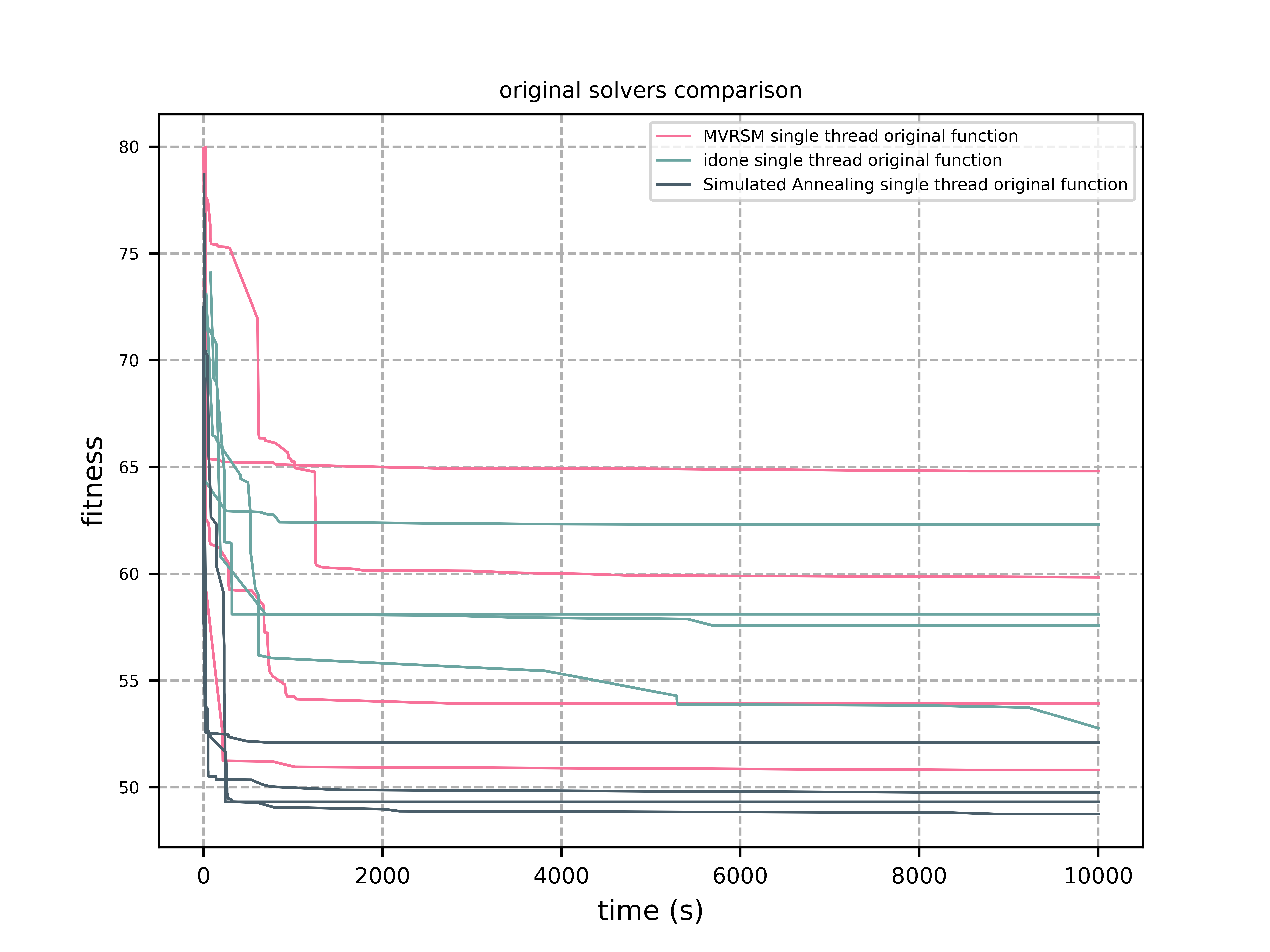
Next, look at how the standard fcmaes optimizers perform in the same single-threaded setting. We use the Python wrappers for these three algorithms implemented with Eigen/C++:

Differential Evolution.
BiteOpt from Aleksey Vaneev, see also BiteOpt.
CMA-ES.

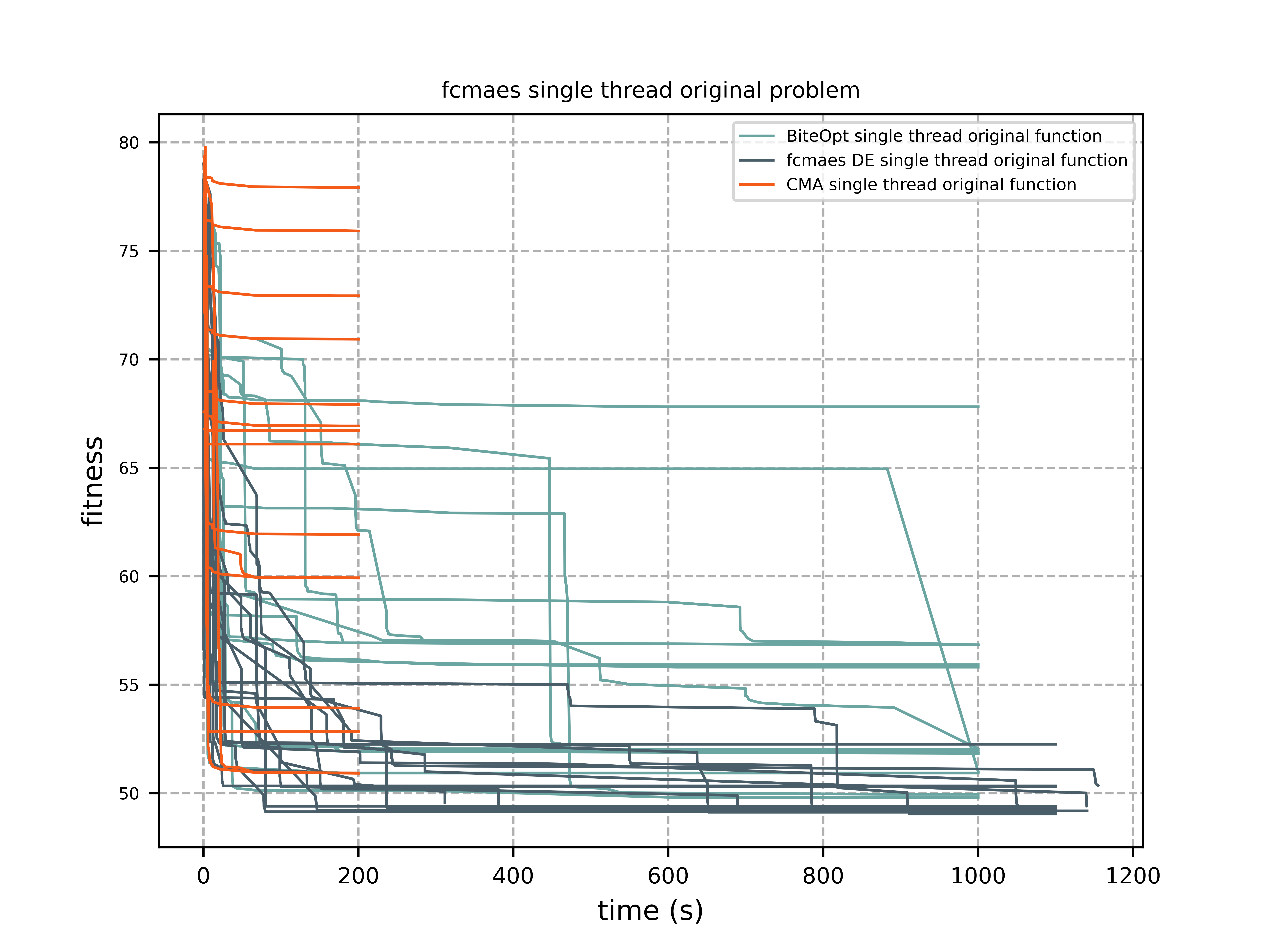
The fcmaes CMA variant terminates quickly, but its results are inconsistent.

fcmaes also supports parallel retry for optimization algorithms. Now apply 32 optimization runs in parallel with retry.py:

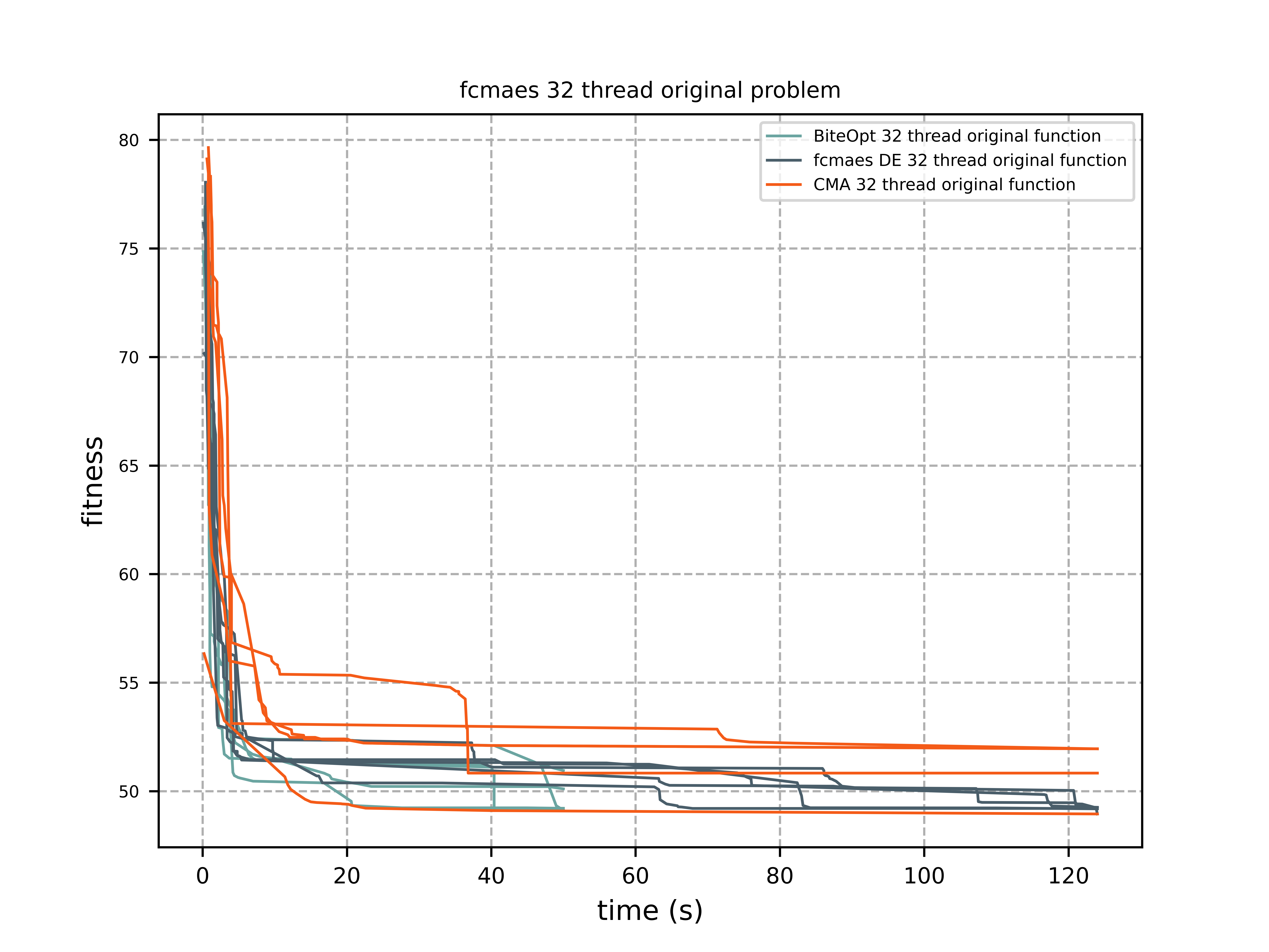
The original algorithms are clearly outperformed. Even CMA-ES works well in this parallel-retry setting.

UPDATE: Mixed integer support

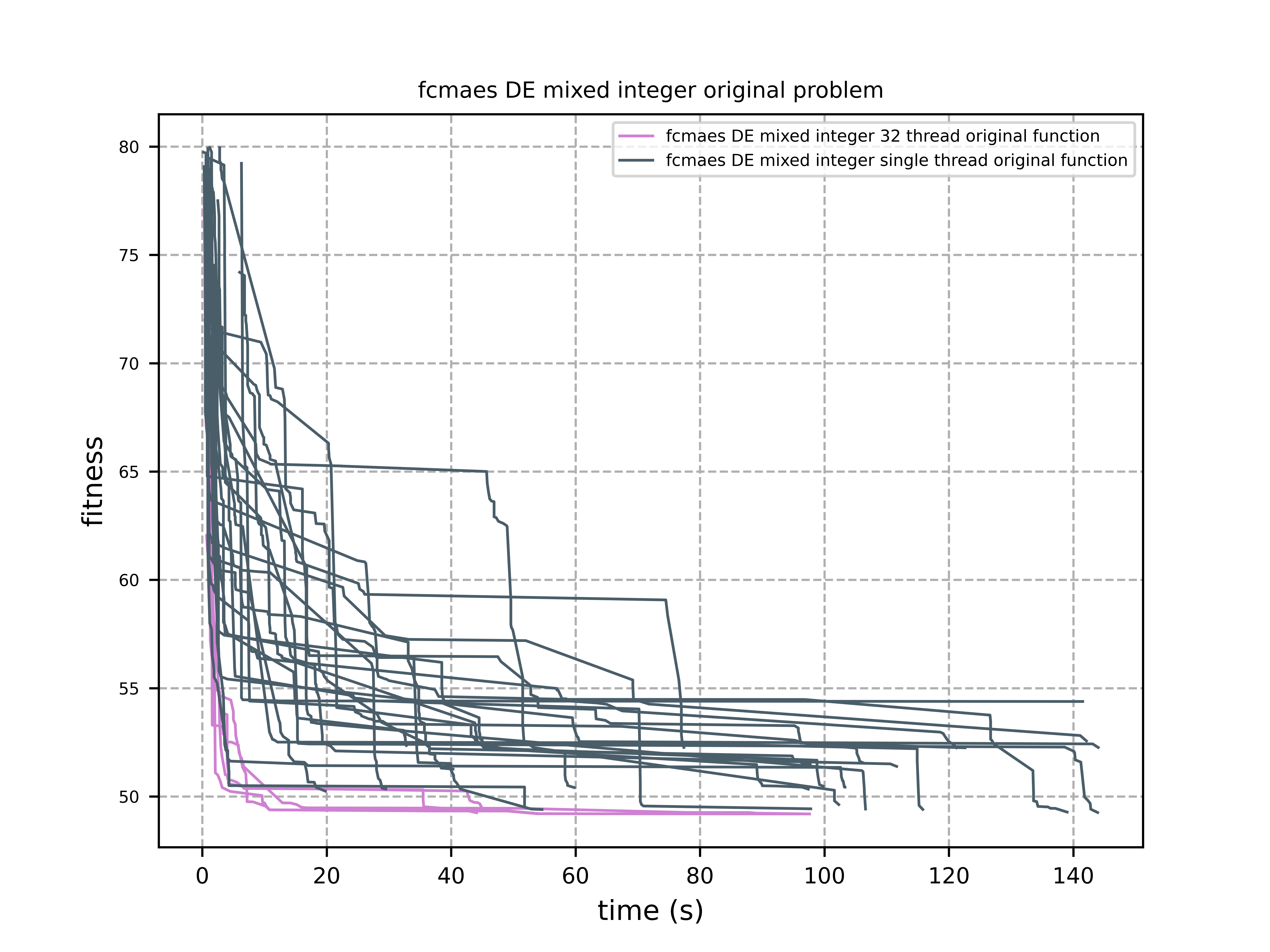
Both the Differential Evolution and multiobjective DE/NSGA (MODE) algorithms were updated:

Both algorithms now support mixed-integer optimization directly. With the new boolean array parameter ints, you can mark which variables are discrete integer variables, and convergence becomes much faster. This works in both the Python and C++ variants. ints = [True, True, False] means, for example, that the first two variables are discrete. Using np.argsort(x) with continuous variables for sequences, as shown below, is still a valid option. But that trick does not work when the same discrete value can appear in different variables. The original problem is now solvable in about 10 seconds using multiple threads.

fcmaes DE mixed integer original problem

An alternative implementation of the objective function

The new implementation (noisy_tsp.py) uses numba to speed up the objective-function evaluation significantly:

@njit(fastmath=True)
def evaluate_tsp(x, W, d, noise_factor, iter_num):
    robust_total_route_length = 0
    order = np.argsort(x) + 1
    for _ in range(iter_num):
        total_route_length = 0
        total_route_length += W[0, order[0]] + np.random.random() * noise_factor
        total_route_length += W[order[d-1], 0] + np.random.random() * noise_factor
        for i in range(d-1):
            total_route_length += W[order[i], order[i+1]] + np.random.random() * noise_factor
        robust_total_route_length = max(total_route_length, robust_total_route_length)
    return robust_total_route_length

This version uses np.argsort(x) to determine the visit order. The first city is fixed, so the number of argument variables is the number of cities N minus one. That is one variable more, but it works much better with continuous optimization algorithms. We use the same idea in Scheduling and JobShop.

Applying the standard fcmaes optimization algorithms to the modified objective function

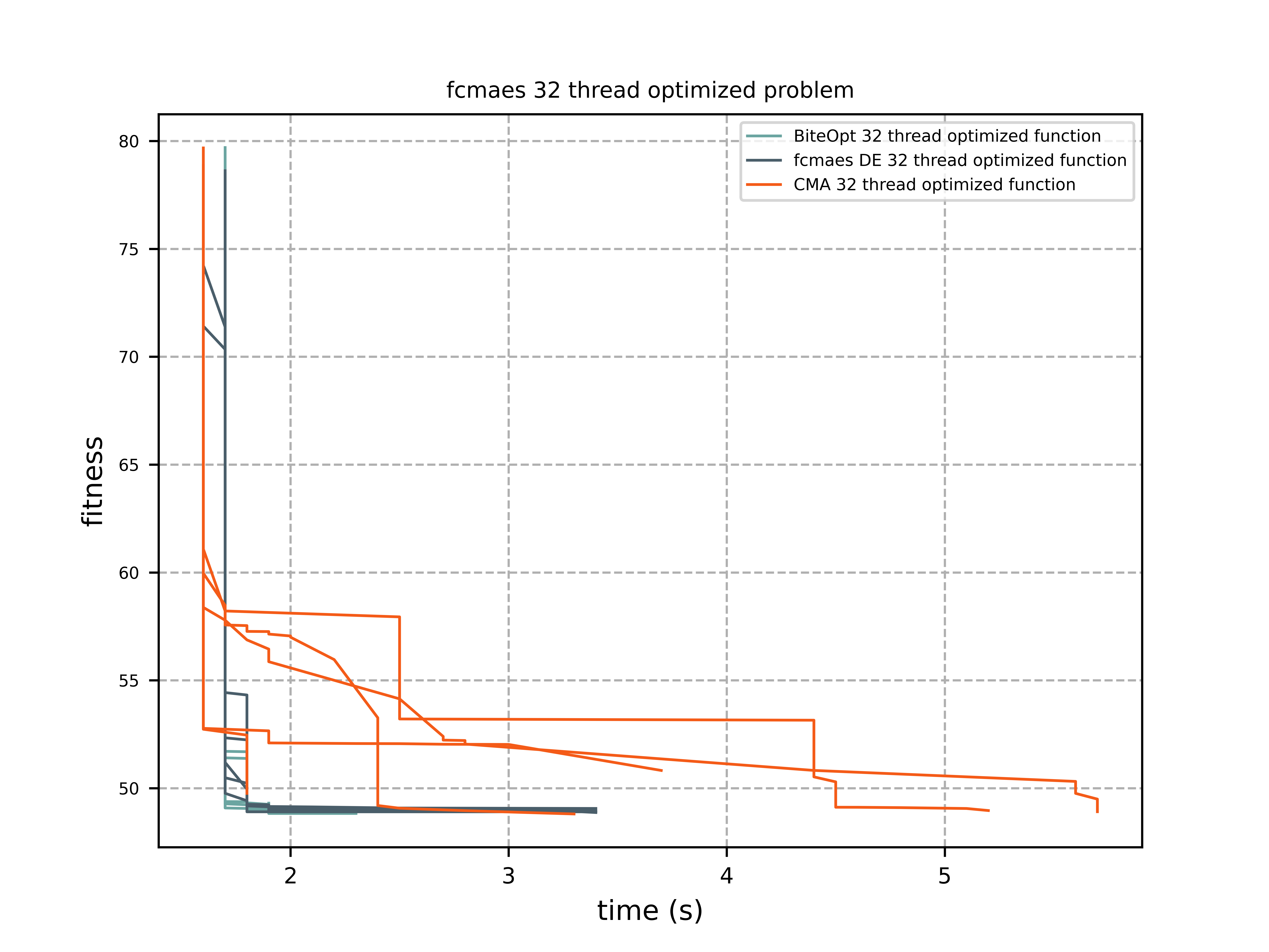
gives a solution time of about 2 seconds. Even for CMA-ES it is only about 5 seconds.

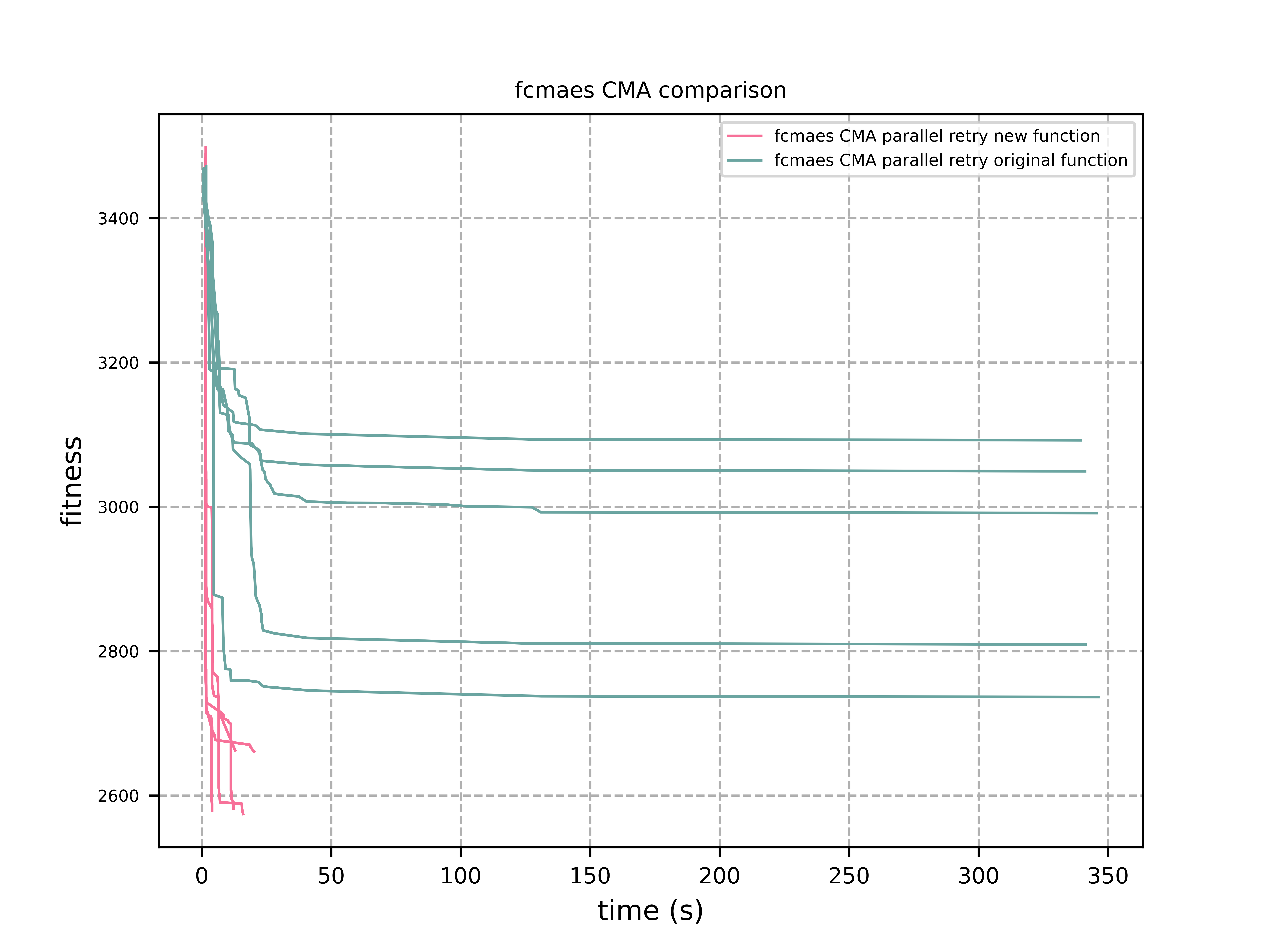
The following table compares the number of function evaluations per second for all algorithms and objective-function variants. numba and the design of the new implementation increase throughput by about a factor of 100. They also improve convergence.

Table 1. Evaluations / second on CPU AMD 5950x
algorithm	problem	evals/sec	used threads
idone	original	13	1
MSVRM	original	23	1
CMA	original	271	1
SA	original	335	1
BiteOpt	original	11800	32
fcmaes-CMA	original	11600	32
BiteOpt	numba based	1150000	32
fcmaes-CMA	numba based	1190000	32

Increasing the noise

What happens if we increase the noise? The next experiment uses the symmetric TSP gr17. This time we set noise_factor=50. According to TSP-solutions the shortest path without noise has length 2085.

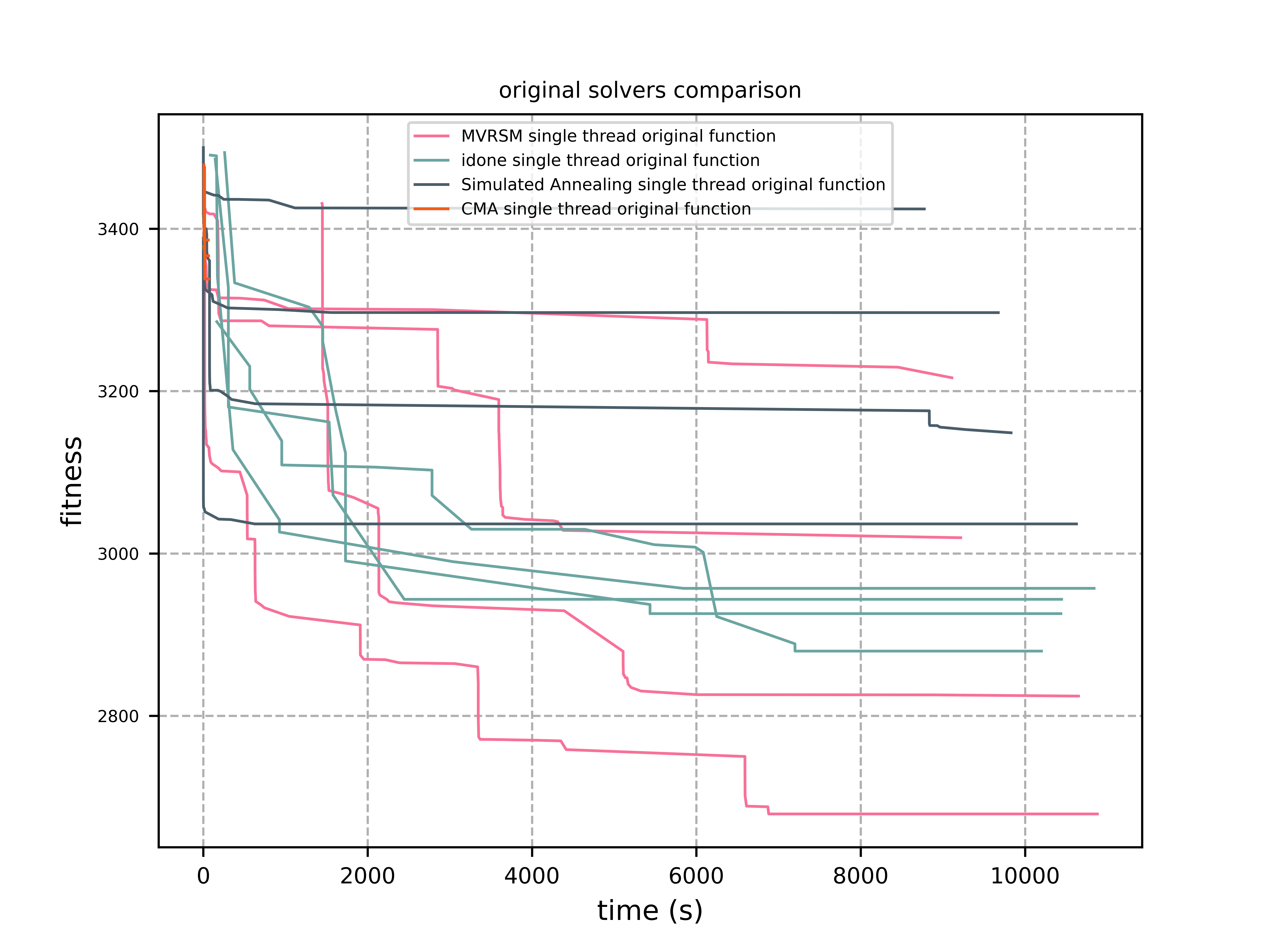
The CMA algorithm shown here is not the one from fcmaes, but the original one:

CMA-ES

The CMA results are hard to see because the run ends with "termination on tolstagnation" after about 8000 function evaluations. The default termination criteria do not seem to work well for this TSP problem. As we will see, that is not a problem with CMA-ES itself.

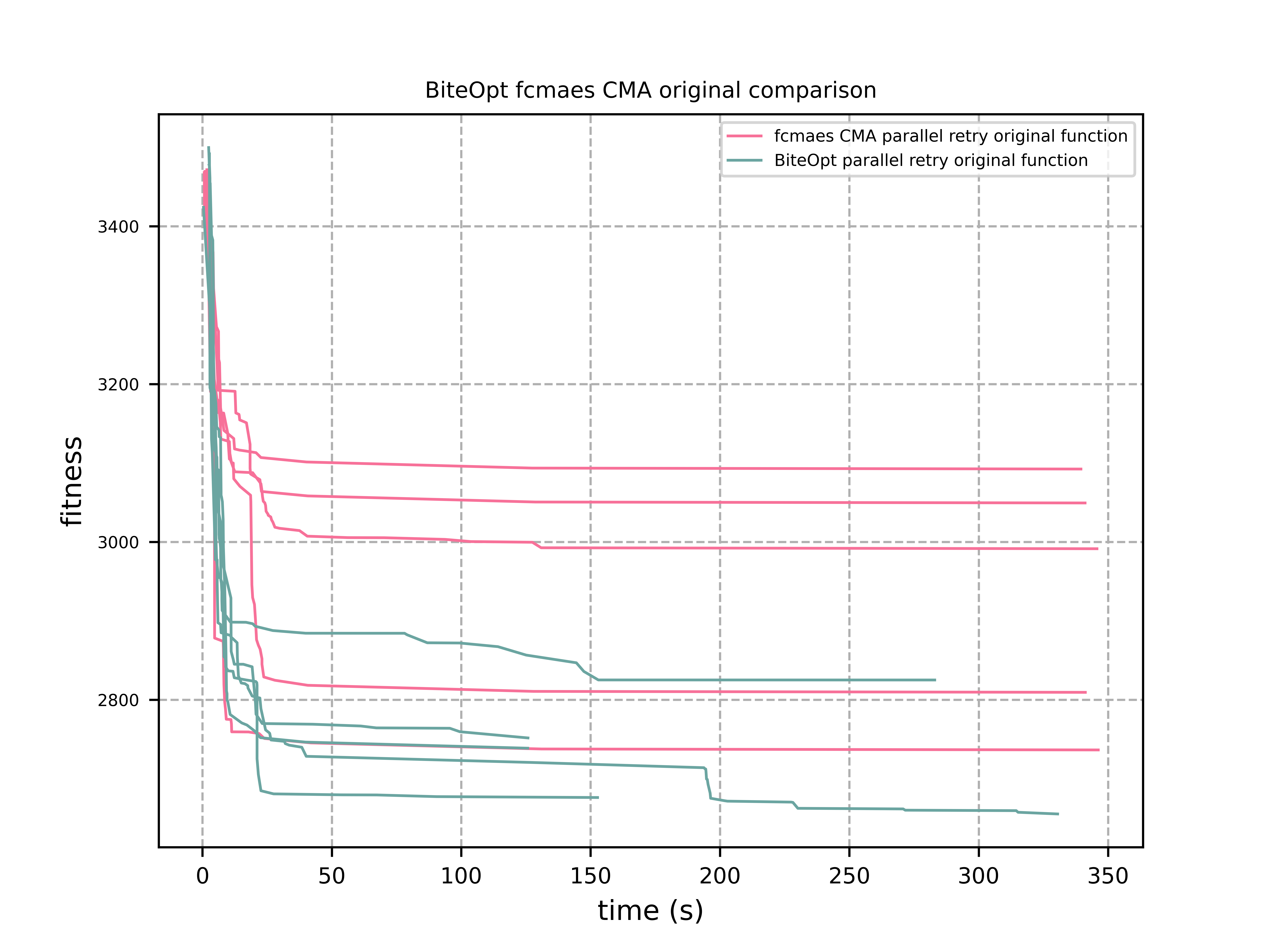
CMA-ES is based on pycma from Nikolaus Hansen.

Here are the results for fcmaes-CMA, not the original one, and BiteOpt, both using all 32 threads of the processor:

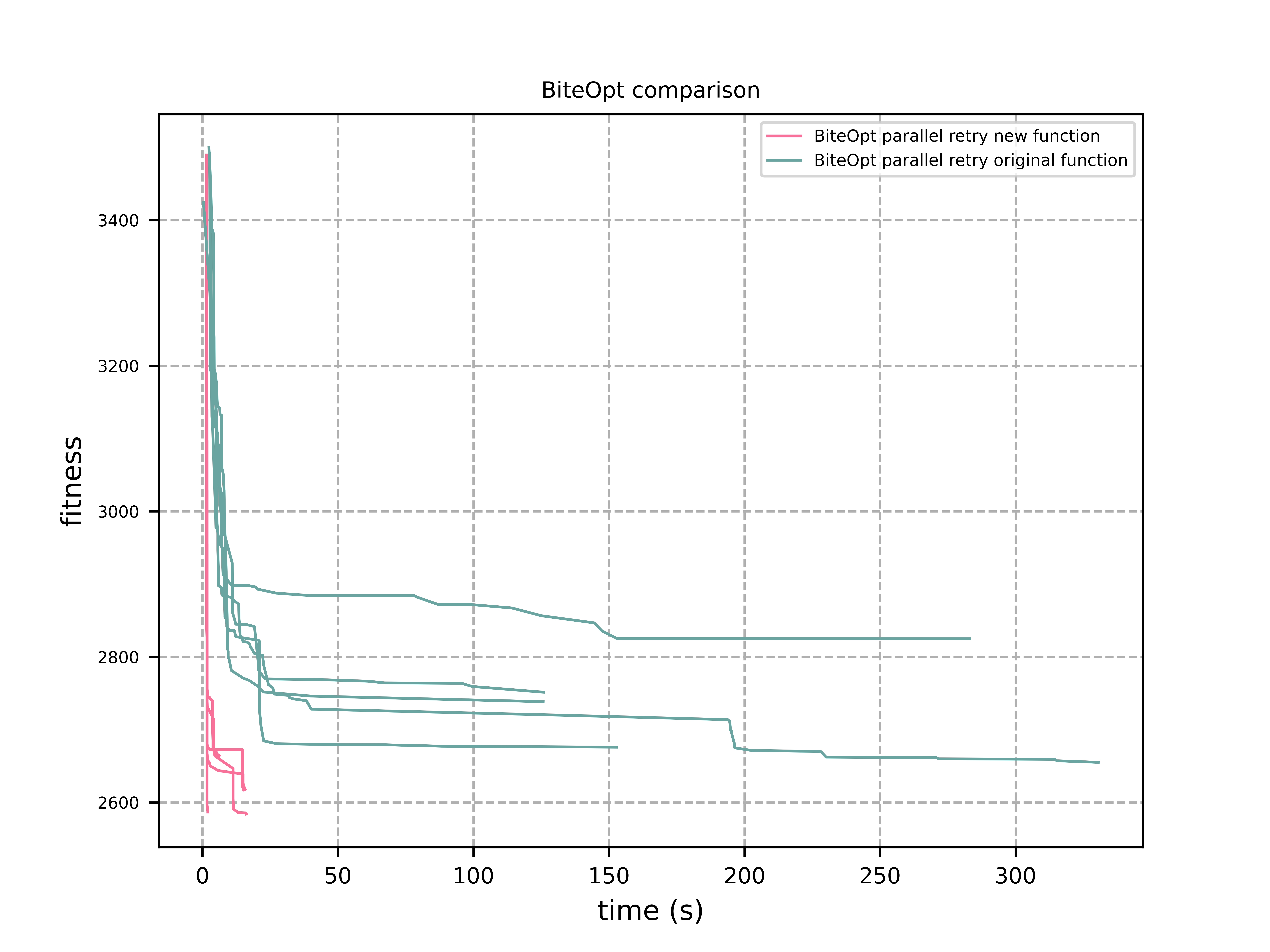
Finally, we can compare the two objective-function implementations directly with the same optimization algorithm. In addition to the speedup in evaluations per second, both algorithms also find better robust tours.

Conclusion

We need to be careful when implementing an objective function for a specific problem. The representation with the fewest variables does not always win. Use numba whenever possible for the time-critical parts. BiteOpt or Differential Evolution, especially with parallel retry, are good choices to try early when the problem is single-objective and unconstrained, or when constraints can be expressed with a weighted-sum approach. Algorithms with high overhead such as IDONE and MSVRM should be reserved for very expensive objective functions. Noisy TSP can be evaluated at nearly 1.2 million evaluations per second, so it clearly does not belong in that category.

One more noisy TSP problem

Now look at ai-for-tsp-competition, which contains the Python code for a machine-learning competition on another TSP variant called TD-OPSWTW. Results and details of this variant are described in BliekEtAl2021:

"The stochastic travel times between locations are only revealed as the salesman travels in the network. The salesman starts from a depot and must return to the depot at the end of the tour. Moreover, each node (customer) in the network is assigned a prize, representing how important it is to visit a given customer on a given tour. Each node has associated time windows. We consider that a salesman may arrive earlier at a node without compromising its prize, but the salesman must wait until the opening time to serve the customer. Lastly, the tour must not violate a total travel time budget while collecting prizes in the network. The goal is to collect the most prizes in the network while respecting the time windows and the total travel time of a tour allowed to the salesman."

We focus on the first task from the paper. A specific 65-node instance of this TSP must be solved with machine-learning techniques. Now suppose we are organizing the competition and want to assess how competitive machine learning really is for this problem. We can compare the winning results with a pure optimization-based approach.

As with the first TSP problem above, we do the following:

apply numba to speed up the evaluation of a tour,
formulate an objective function that is fast to evaluate while still accurate enough for the final test, which here is the average of 10000 noisy tour evaluations,
apply the BiteOpt optimizer with parallel retry.

Speeding up the evaluation of a tour (numbafication)

The central routine for evaluating a given tour is tour_check. We need to adapt it:

from numba import njit

def tour_check(tour, x, time_matrix, maxT_pen, tw_pen, n_nodes):
    return tour_check_numba(np.array(tour, dtype=np.int32), np.array(x, dtype=np.float32),
                            np.array(time_matrix, dtype=np.int32), maxT_pen, tw_pen, n_nodes)

@njit(fastmath=True)
def tour_check_numba(tour, x, time_matrix, maxT_pen, tw_pen, n_nodes):

numba is very strict about argument array types, so we add a wrapper that converts the inputs to float32 and int32. That small change already gives about an 8x speedup for tour evaluation.

Objective function for TD-OPSWTW

The fitness object that represents the objective function for optimization receives an Env object representing a problem instance.

Progress is monitored with mp.RawValue variables, which share values between processes.
We set the bounds of all continuous variables to [0,1]. In solution, these values are converted into an integer tour using the np.argsort sorting trick.
value computes the minimum or average score over n calls to check_solution, which gives a noisy tour evaluation. For small n, the minimum is the more reliable value.
The objective function itself __call__ uses value with increasing n to compute the final tour evaluation. This is a compromise between accuracy and performance. For low n, penalized noisy values may be missed. For good candidates we therefore increase n, and this works with n=10000, which is used for the final test.
The optimizer can still find noisy outliers that look worse when evaluated again. We therefore use n=100000 in the end, because n=10000 inside the objective function was not reliable enough.

from scipy.optimize import Bounds
import time, math
import ctypes as ct
import multiprocessing as mp
from fcmaes.optimizer import logger, Bite_cpp, dtime
from fcmaes import retry

class fitness:

    def __init__(self, env):
        self.evals = mp.RawValue(ct.c_long, 0)  # writable across python processes
        self.best_y = mp.RawValue(ct.c_double, math.inf)
        self.t0 = time.perf_counter()
        self.env = env
        self.d = env.n_nodes

    def bounds(self):
        return Bounds(np.zeros(self.d), np.array([1]*self.d))

    def value_min(self, sol, n):
        val = math.inf
        for _ in range(n):
            _, rewards, pen, _ = self.env.check_solution(sol)
            val = min(val, rewards + pen)
        return val

    def value(self, sol, n):
        if n < 1000: # for small n take the minimum instead
            return self.value_min(sol, n)
        val = 0
        for _ in range(n):
            _, rewards, pen, _ = self.env.check_solution(sol)
            val += rewards + pen
        return val/n

    def solution(self, x): # disjoined all locations
        return [1] + [int(xi) for xi in (np.argsort(x) + 1)]

    def __call__(self, x):
        self.evals.value += 1
        sol = self.solution(x)
        n = 10
        while n <= 100000:
            y = -self.value(sol, n)
            if y >= self.best_y.value:
                return y
            n *= 10
        if y < self.best_y.value:
            self.best_y.value = y
            logger().info("evals = {0}: time = {1:.1f} y = {2:.5f} x= {3:s}"
                  .format(self.evals.value, dtime(self.t0), y, str(sol)))
        return y

    def optimize(self):
        self.bestY = 1E99
        self.bestX = []
        ret = retry.minimize(self, self.bounds(), optimizer=Bite_cpp(200000,M=16,stall_iterations=3), num_retries=32)
        sol = self.solution(ret.x)
        num = 10000
        logger().info("val" + str(num) + " = " + str(self.value(sol, num)))
        return sol

if __name__ == '__main__':

    env = Env(n_nodes=65, seed=6537855)
    sol = fitness(env).optimize()

A typical output is:

evals = 32: time = 12.7 y = 72.28609 x= [1, 28, 44, 36, 4, 17, 54, 40, 19, 45, 1, 14, 37, 12, 6, 11, 34, 13, 52, 38, 62, 60, 42, 5, 8, 61, 63, 35, 33, 65, 2, 30, 53, 27, 48, 56, 20, 26, 3, 25, 55, 10, 22, 59, 18, 58, 46, 57, 24, 29, 16, 49, 64, 47, 51, 50, 21, 31, 39, 32, 23, 43, 9, 41, 15, 7]
evals = 36: time = 12.7 y = 67.64000 x= [1, 34, 20, 18, 63, 1, 26, 43, 10, 36, 24, 44, 56, 62, 3, 17, 42, 27, 25, 41, 21, 64, 12, 54, 31, 22, 7, 9, 16, 28, 4, 60, 11, 45, 2, 23, 32, 39, 51, 8, 46, 29, 61, 65, 47, 35, 14, 40, 13, 52, 33, 55, 57, 48, 53, 38, 6, 19, 58, 15, 59, 50, 37, 5, 49, 30]
evals = 56: time = 12.7 y = 66.42925 x= [1, 36, 13, 56, 62, 17, 1, 55, 30, 46, 25, 53, 34, 10, 38, 27, 7, 9, 54, 64, 28, 22, 57, 23, 31, 2, 6, 18, 47, 58, 44, 39, 50, 43, 42, 8, 12, 65, 32, 37, 61, 5, 24, 21, 26, 14, 48, 11, 15, 63, 33, 45, 16, 52, 51, 59, 35, 41, 49, 20, 4, 19, 40, 3, 60, 29]
...
evals = 930879: time = 142.3 y = -5.00259 x= [1, 45, 5, 44, 47, 42, 2, 46, 9, 22, 7, 4, 24, 30, 40, 48, 1, 41, 39, 43, 49, 52, 51, 38, 53, 54, 55, 56, 57, 58, 59, 60, 61, 62, 63, 50, 37, 33, 35, 3, 6, 8, 10, 11, 12, 13, 14, 15, 16, 17, 18, 19, 20, 23, 25, 26, 27, 28, 29, 31, 32, 64, 34, 36, 65, 21]
...
evals = 6060526: time = 474.5 y = -11.20464 x= [1, 32, 45, 55, 49, 47, 41, 5, 23, 57, 6, 16, 2, 42, 46, 60, 11, 33, 43, 64, 13, 19, 29, 9, 22, 65, 7, 35, 62, 63, 4, 24, 30, 40, 48, 1, 17, 56, 26, 3, 36, 27, 37, 10, 34, 8, 58, 61, 39, 12, 25, 59, 44, 52, 15, 14, 28, 51, 54, 20, 18, 31, 53, 50, 38, 21]
...
evals = 6186914: time = 492.6 y = -11.31701 x= [1, 32, 45, 55, 5, 49, 41, 47, 44, 23, 6, 57, 16, 33, 60, 46, 42, 2, 11, 64, 19, 43, 13, 29, 65, 9, 22, 35, 7, 62, 63, 4, 24, 30, 40, 48, 1, 21, 8, 61, 14, 50, 54, 17, 38, 59, 27, 28, 26, 36, 15, 58, 20, 56, 34, 37, 18, 12, 31, 51, 10, 25, 3, 53, 39, 52]
evals = 6232151: time = 501.8 y = -11.31998 x= [1, 32, 45, 55, 5, 49, 41, 47, 44, 23, 6, 57, 16, 33, 2, 60, 46, 42, 11, 64, 19, 43, 13, 29, 65, 9, 22, 35, 7, 62, 63, 4, 24, 30, 40, 48, 1, 21, 8, 61, 14, 50, 54, 17, 38, 59, 27, 28, 26, 36, 15, 58, 20, 56, 34, 37, 18, 12, 31, 51, 10, 25, 3, 53, 39, 52]
evals = 6260525: time = 518.0 y = -11.32000 x= [1, 32, 45, 55, 5, 49, 41, 47, 44, 23, 6, 57, 16, 33, 2, 60, 46, 42, 11, 64, 19, 43, 13, 29, 65, 9, 22, 35, 7, 62, 63, 4, 24, 30, 40, 48, 1, 21, 8, 61, 14, 50, 54, 17, 38, 59, 27, 28, 26, 36, 15, 56, 58, 20, 34, 37, 18, 12, 31, 51, 10, 25, 3, 53, 39, 52]

val10000 = 11.319876970495283

Conclusion

The machine-learning approach and the optimization approach both reach almost the same result: 11.32. Optimization reaches 11.20 consistently after about 400-500 seconds, but can need up to 1800 seconds to reach 11.32 for the TD-OPSWTW instance from the competition on an AMD-5950x 16-core CPU.

Even with 10000 evaluations there is still some noise. That is why the final test can be slightly worse, even though we use 100000 evaluations inside the objective function. Pure optimization therefore looks like a valid alternative for TD-OPSWTW and other realistic TSP variants.

Compare it yourself with the machine-learning-based approach of one of the winners: https://github.com/mustelideos/td-opswtw-competition-rl . Which solution do you prefer?