

Vehicle Routing
This tutorial
-
Is related to Vehicle Routing
-
Shows an alternative implementation using numba.
-
Compares different optimization algorithms applied to this problem.
-
Extends the problem by adding a second objective: The maximal vehicle capacity.
All results were produced on a 16 core / 32 thread AMD CPU 5950x. The code for this tutorial is here: routing.py
Problem Statement
The original problem statement from Vehicle Routing:
"Delivery companies every day need to deliver packages to many different clients. The deliveries are accomplished using an available fleet of vehicles from a central warehouse. The goal of this exercise is to design a route for each vehicle so that all customers are served, and the number of vehicles (objective 1) along with the total traveled distance (objective 2) by all the vehicles are minimized. In addition, the capacity of each vehicle should not be exceeded (constraint 1)"
Due date, service time, and ready time are ignored.
Minimizing the number of vehicles and minimizing total travel distance are not competing objectives here. As a result, the Pareto front always contains a single element. Therefore we
-
Solve the single-objective variant independent of the vehicle number.
-
Define a 2-objective variant maximizing the vehicle number. This works, but it does not make much sense.
-
Define a useful 2-objective variant optimizing total travel distance and vehicle capacity.
Motivation
Vehicle Routing implements the vehicle routing problem with a custom individual encoding and decoding, together with custom mutation and crossover operations. This approach has several drawbacks:
-
All custom code must be adapted when the problem changes or is extended, for example to include due date, service time, or ready time. If we reduce the amount of problem-specific code, adaptation becomes much easier.
-
Defining additional / alternative objectives is difficult.
-
Low performance of the fitness function evaluation.
-
No automated parallelization.
If you execute the given code
runAlgo.py
with the provided parameterization, you do not get good results for the predefined vehicle
capacity=70. I therefore changed numGen = 20000 (default is 200) and ran the code manually 16 times in parallel
to use the CPU cores. After a few minutes I got:
Best individual is [12, 14, 16, 15, 19, 18, 23, 25, 24, 20, 17, 13, 11, 10, 1, 2, 4, 3, 5, 8, 9, 6, 7, 21, 22]
Number of vechicles required are 7.0
Cost required for the transportation is 378.5564153198204
  Vehicle 1's route: 0 - 12 - 14 - 16 - 0
  Vehicle 2's route: 0 - 15 - 19 - 18 - 0
  Vehicle 3's route: 0 - 23 - 25 - 24 - 20 - 0
  Vehicle 4's route: 0 - 17 - 13 - 11 - 10 - 0
  Vehicle 5's route: 0 - 1 - 2 - 4 - 3 - 5 - 0
  Vehicle 6's route: 0 - 8 - 9 - 6 - 7 - 0
  Vehicle 7's route: 0 - 21 - 22 - 0

...

Best individual is [5, 3, 4, 7, 13, 17, 22, 12, 14, 16, 15, 19, 18, 1, 2, 6, 21, 10, 11, 9, 8, 23, 25, 24, 20]
Number of vechicles required are 7.0
Cost required for the transportation is 404.1737778339401
  Vehicle 1's route: 0 - 5 - 3 - 4 - 7 - 0
  Vehicle 2's route: 0 - 13 - 17 - 22 - 0
  Vehicle 3's route: 0 - 12 - 14 - 16 - 0
  Vehicle 4's route: 0 - 15 - 19 - 18 - 0
  Vehicle 5's route: 0 - 1 - 2 - 6 - 0
  Vehicle 6's route: 0 - 21 - 10 - 11 - 9 - 8 - 0
  Vehicle 7's route: 0 - 23 - 25 - 24 - 20 - 0
The standard deviation of the results was high. I got several results > 400. This means:
-
Even with 20000 generations you have to be lucky.
-
Parallelization is manual, and you have to inspect all results to find a good one.
-
But at least I found a good result this way.
Let us see if we can do better.
Fast Fitness Function
The first step is a fast fitness function using numba. In combination with parallelization, this enables an evaluation rate > 1E6 / second. That makes single-objective optimization possible in less than 2 seconds, and multi-objective optimization in less than a minute.
@njit(fastmath=True)
def fitness_(seq, distance, demands, capacity):
    n = len(seq)
    seq += 1
    sum_demand = 0
    sum_dist = 0
    last = 0
    vehicles = 1
    for i in range(n+1):
        customer = seq[i] if i < n else 0
        demand = demands[customer]
        if sum_demand + demand > capacity:
            # end vehicle tour, return to base
            sum_dist += distance[last, 0]
            sum_demand = 0
            vehicles += 1
            last = 0
        # go to customer
        sum_demand += demand
        sum_dist += distance[last, customer]
        last = customer
    return np.array([-float(vehicles), sum_dist])
We use an encoding very similar to
Vehicle Routing. The input is a
sequence of unique integer vehicle indices. The vehicle tours are then determined "on the fly" when
the capacity limit is exceeded. Up to this point we do not need classes, because this is easier with numba.
We also leave all optimization-related work to predefined algorithms from the fcmaes library.
There is no need to define problem-specific mutation and crossover operations.
We define a Routing class that hosts both the multi-objective and the single-objective variants of the
fitness function, together with the demands array and the distance matrix. As boundaries we use
the [0,1] interval and the np.argsort(x) trick to convert the continuous argument vector x into a
sequence of unique integer indices. This lets us apply standard continuous optimization algorithms.
class Routing():
    def __init__(self, filename, capacity):
        self.capacity = capacity
        self.demands, self.distance = parse(filename)
        self.dim = len(self.demands) - 1
        self.bounds = Bounds([0]*self.dim, [1]*self.dim)

    def fitness(self, x):  # returns number of vehicles and cost
        return fitness_(np.argsort(x), self.distance, self.demands, self.capacity)

    def fitness_so(self, x): # returns the cost only
        return fitness_(np.argsort(x), self.distance, self.demands, self.capacity)[1]
This is much simpler than defining problem-specific crossover and mutation operations. So it is fair to ask: why use this approach at all? One reason is pedagogical. You get involved in the inner workings of the optimization process. Another is that the power of continuous optimization for discrete problems is often underestimated. There are not many open-source libraries that provide fast implementations of state-of-the-art algorithms and also parallelize well across many CPU cores.
For larger instances or more complex problem variants, you should definitely use a fast fitness function implementation and an optimizer that uses all CPU cores.
Single-Objective Optimization
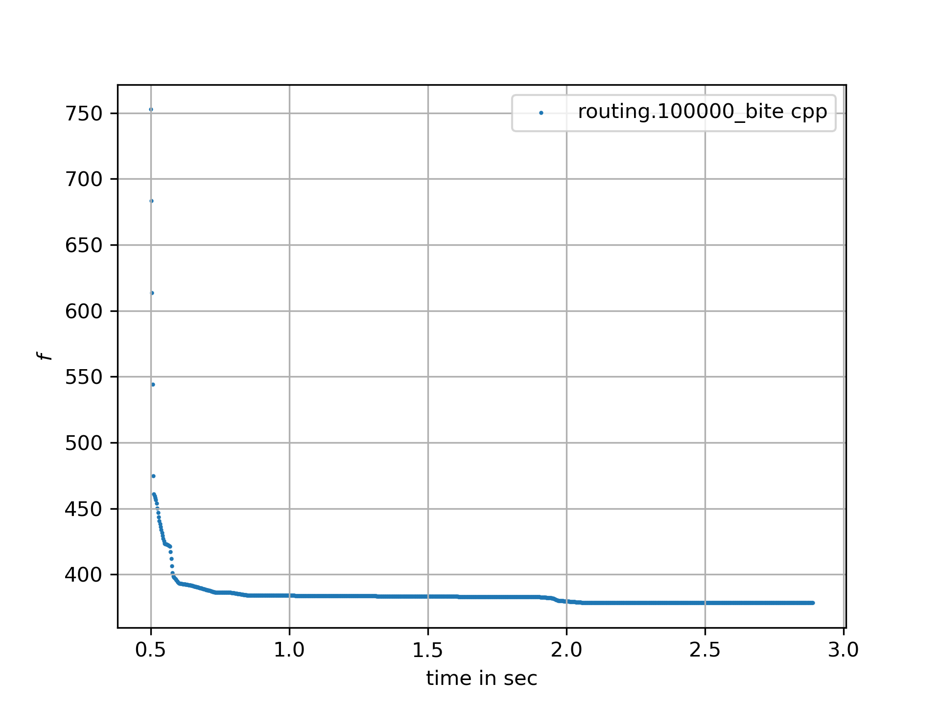
We use a standard wrapper around the single-objective fitness function to monitor the progress
of the parallel optimization. We then use the minimize_plot function, which not only optimizes,
but also produces a plot of the progress over time.
def optimize_so(filename, capacity, opt, num_retries = 320):
    routing = Routing(filename, capacity)
    name = "routing." + str(opt.max_evaluations)
    ret = retry.minimize_plot(name, opt, wrapper(routing.fitness_so),
                               routing.bounds, num_retries = num_retries, logger=logger())
    routing.dump(np.argsort(ret.x), ret.fun)

capacity = 70
popsize = 128
max_evaluations = 100000

optimize_so(filename, capacity, Bite_cpp(max_evaluations))
#optimize_so(filename, capacity, Crfmnes_cpp(max_evaluations,popsize=popsize))
#optimize_so(filename, capacity, de_cma(max_evaluations,popsize=popsize))
#optimize_so(filename, capacity, De_cpp(max_evaluations,popsize=popsize))
We propose four different single-objective algorithms. BiteOpt is the best choice here. You do not need to tune the algorithm, because it supports "auto-configuration". The three other choices also produce good results very quickly.
Even when coding your problem-specific operations, such as crossover and mutation, in Assembler,
it will not be easy to beat this result with capacity=70:
tour  [23, 25, 24, 20, 22, 21, 16, 14, 12, 17, 13, 11, 10, 1, 2, 4, 3, 5, 7, 6, 9, 8, 15, 19, 18]
y  378.55641531982036
vehicle  1 tour [0, 23, 25, 24, 20, 0] demands 70.0 distance 34.242640687119284
vehicle  2 tour [0, 22, 21, 0] demands 40.0 distance 58.606204774901286
vehicle  3 tour [0, 16, 14, 12, 0] demands 70.0 distance 141.99635904571358
vehicle  4 tour [0, 17, 13, 11, 10, 0] demands 70.0 distance 213.37888633392356
vehicle  5 tour [0, 1, 2, 4, 3, 5, 0] demands 70.0 distance 255.79872525207853
vehicle  6 tour [0, 7, 6, 9, 8, 0] demands 70.0 distance 297.1455635058531
vehicle  7 tour [0, 15, 19, 18, 0] demands 70.0 distance 378.55641531982036
Multi-Objective Optimization
Minimizing the number of vehicles is not a competing goal here, so it makes more
sense to compare results for different vehicle capacity settings.
We add a new input variable that defines the capacity of all vehicles, set its
boundaries to [40, 500], and return it as an objective together with the cost.
class Routing():
    def __init__(self, filename, capacity):
        ..
        self.bounds_capacity = Bounds([40] + [0]*(self.dim), [500] + [1]*self.dim)

    def fitness_capacity(self, x):
        y = fitness_(np.argsort(x[1:]), self.distance, self.demands, x[0])
        return np.array([x[0], y[1]])

def optimize_capacity(filename, popsize, max_evaluations, num_retries = 640):
    routing = Routing(filename, 0)
    x, y = modecpp.retry(mode.wrapper(routing.fitness_capacity, 2, interval = 10000000), 2, 0,
                 routing.bounds_capacity, popsize = popsize,
                 max_evaluations = max_evaluations,
                 nsga_update=True, num_retries = num_retries)
    pname = "routing." + str(popsize) + "." + str(max_evaluations)
    np.savez_compressed(pname, xs=x, ys=y)
    moretry.plot(pname, 0, x, y, all=False, interp=True)#, plot3d=True)
    routing.dump(np.argsort(x[-1][1:]), y[-1], y[-1][0])
The Pareto front shows that we could save some cost by increasing vehicle capacity.
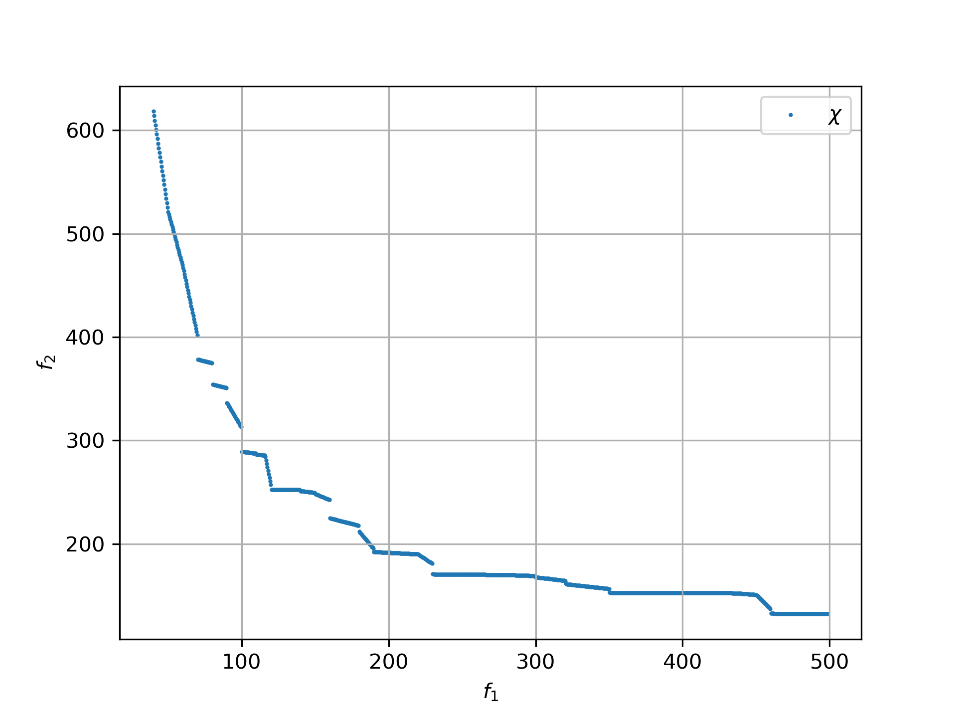
Pareto front:
[40.0, 618.3907115437548] [40.0, 0.47093, 0.49844, 0.39375, 0.49976, 0.40218, 0.55715, 0.35621, 0.64084, 0.58421, 0.67753, 0.65804, 0.14671, 0.69748, 0.13105, 0.17688, 0.19121, 0.00453, 0.05082, 0.05447, 0.94852, 0.74455, 0.83638, 0.73859, 0.88992, 0.78497]
...
[70.00009380697202, 378.55641531982036] [70.00009, 0.36217, 0.36317, 0.43649, 0.40161, 0.45219, 0.48159, 0.46036, 0.57442, 0.5652, 0.34037, 0.31426, 0.00848, 0.27692, 0.09889, 0.15106, 0.13469, 0.2391, 0.22958, 0.20722, 0.77681, 0.82719, 0.79605, 0.60043, 0.74514, 0.68503]
[80.0000014820427, 366.38436101504595] [80.0, 0.65229, 0.63874, 0.66709, 0.63649, 0.68901, 0.52217, 0.76201, 0.5186, 0.47152, 0.35066, 0.41905, 0.34831, 0.38981, 0.32899, 0.21383, 0.31939, 0.26637, 0.2593, 0.29995, 0.99657, 0.84268, 0.96297, 0.80748, 0.93927, 0.90448]
...
460.01098236218775, 132.12162500340892] [460.01098, 0.74831, 0.73675, 0.88968, 0.72019, 0.89847, 0.7128, 0.91608, 0.68842, 0.70344, 0.51361, 0.51281, 0.49429, 0.19855, 0.38483, 0.28595, 0.309, 0.24909, 0.26547, 0.27641, 0.00253, 0.02819, 0.0651, 0.1843, 0.11321, 0.14182]

tour  [20, 21, 22, 24, 25, 23, 13, 17, 18, 19, 15, 16, 14, 12, 11, 10, 8, 9, 6, 4, 2, 1, 3, 5, 7]
y  [460.01098236 132.121625  ]
vehicle  1 tour [0, 20, 21, 22, 24, 25, 23, 13, 17, 18, 19, 15, 16, 14, 12, 11, 10, 8, 9, 6, 4, 2, 1, 3, 5, 7, 0] demands 460.0 distance 132.12162500340892