fcmaes - a Python 3 gradient-free optimization library

Reactive Programming and Real World Optimization

This tutorial:

discusses the relation between reactive programming and optimization with parallel fitness evaluations.
applies parallel fitness evaluation to a live hospital management problem.
shows that parallel fitness evaluation increases the number of evaluations.
shows that the advantage of surrogates, approximations, or gaussian processes can disappear as the evaluation count grows.

Reactive Programming

Recently reactive programming has gained a lot of traction. Reactive frameworks such as Spring Reactive are adopted more and more widely.

Real World Optimization

Real-world optimization has recently become a major focus in optimization research. One example is the Hospital Management Problem, which studies hospital management during a pandemic. Real-world optimization usually involves expensive simulation-based objective functions.

How are these connected?

A reactive program sees its environment as sequences of asynchronous events that it receives and emits. In optimization, this means an optimizer emits a stream of argument vectors and receives a stream of results computed by an expensive simulation-based objective function. On the other side there is a reactive function evaluator, which receives argument vectors and emits results.

What is the advantage of reactive programming for optimization?

The function evaluator may decide to:

Spawn separate threads or processes that execute the simulation. See for instance evaluator.py
Spawn separate jobs in a cloud cluster. See for instance OptimizerActivityImpl.java which uses the temporal.io workflow management framework and can optionally distribute tasks (called activities) in a cloud environment.

The Hospital Management Problem spawns Docker runs to execute its hospital simulation. In a kubernetes-based cloud environment this could mean running a kubernetes job that is physically executed on a different CPU or even in a different cluster.

Spawning a separate process or running a kubernetes job is inherently asynchronous. The goal is to speed up optimization by distributing expensive objective function evaluations. But the reactive function evaluator is only one part of the solution. It also needs a reactive counterpart: the optimizer.

Bridging reactive flows and blocking calls

In an ideal world, both sides, the optimizer and the parallel function evaluator, would use a reactive style and avoid blocking calls. In practice, we often have to deal with blocking APIs like this.

A parallel function evaluator can serve as a bridge in both directions:

To the blocking function evaluation: y = fun(x).
To its caller it can provide a blocking API: eval_parallel.

Unfortunately this bridge idea does not work on the optimizer side. An optimizer that expects argument vectors sequentially cannot be parallelized. This is true for all optimizers in solvers.

Backpressure

Backpressure is the "Resistance or force opposing the desired flow of data through software." In optimization, this means there is a limit beyond which parallel objective function evaluation stops making sense. For population-based algorithms, the number of parallel workers should usually not exceed the population size. This limit induces backpressure in the optimization data flow, that is, in the exchange of argument vectors and results. One advantage of reactive frameworks is that they support configurable backpressure limits that can be propagated through a chain of reactive processing flows. In real-world optimization, backpressure defines the rate at which the parallel evaluator receives argument vectors. To evaluate an optimization method, we need results for different backpressure limits, which correspond to different maximum levels of parallelization. Higher backpressure, or more parallelization, usually means a larger population size. That can slow convergence, but it also lowers the chance of getting stuck in a local minimum.

What does that mean for the optimizer?

A reactive optimizer needs an asynchronous, event-based interface. Let’s have a look at how the optimizers in solvers work, for instance CMA:

def f(x):
...
        return r
...
res = fmin(f, x0 / cmascale, sigma0, options=opts)

A synchronous function f is passed to the optimizer fmin, which means the evaluation of f cannot be parallelized. The optimizer expects results in order. Only after one result is returned do we get a new argument vector for evaluation.

In the optimization context, the asynchronous interface we need is known as an ask/tell interface. It is implemented, for instance, in the nevergrad framework. fcmaes supports this interface for its differential evolution and CMA-ES implementations. If multiple objectives and constraints are involved, it also supports it through the MO-DE optimizer, which integrates ideas from DE and NSGA-II.

Providing a reactive or asynchronous interface imposes some restrictions on the optimization:

Mainly population-based algorithms can profit from parallel function evaluation.
Population size should be >= the number of parallel threads, processes, or jobs.

Evaluating surrogate optimization algorithms

ExpensiveOptimBenchmark aims to evaluate surrogate models on real-world problems. But in the real world, when you face such an optimization problem, you would exploit every option to parallelize function evaluation, using multiple cores or even multiple cluster nodes. So surrogate models should be compared to these parallel algorithms, not to sequential ones.

Optimizing the hospital management problem

Suppose we are a hospital manager looking for a solution to the Hospital Management Problem, implemented here: DockerHospitalBenchmark.py See also Competition.

To justify the latest hardware investment, the manager first tries standard optimization methods that can fully use all cores of the newly bought machine.

This is a single-objective problem without separate constraints, so we could use nevergrad or fcmaes. Both support the asynchronous ask/tell interface and parallel function evaluation. Another alternative is ESA’s Pygmo using archipelagos, but this approach needs many function calls and parallel function evaluation does not work out of the box.

Since this is an fcmaes tutorial, our virtual hospital manager chooses fcmaes, although nevergrad would work as well. We need to adapt DockerHospitalBenchmark.py for use with fcmaes:

To monitor progress, we need some variables shared across Python processes, and we wrap evaluate(xs).
We add a method optimize(self, popsize, max_evaluations) that calls the optimizer.
We initialize self.ints, a list of booleans indicating which variables are discrete. This is used by the de algorithm.

Most of the changes are in the super class BaseProblem. We adapt the other classes in the same way. If you are on Linux, you may replace de and cmaes with their C++ counterparts decpp and cmaescpp, which are slightly more efficient.

...
from scipy.optimize import Bounds
from fcmaes import de, cmaes, decpp, cmaescpp
import time
import ctypes as ct
import multiprocessing as mp
from fcmaes.optimizer import logger, dtime
import math

class BaseProblem:

    def __init__(self):
        self.evals = mp.RawValue(ct.c_long, 0)  # writable across python processes
        self.best_y = mp.RawValue(ct.c_double, math.inf) # writable across python processes
        self.t0 = time.perf_counter()

    def bounds(self):
        return Bounds(self.lbs(),self.ubs())

    def fun(self, xs):
        y = self.evaluate(xs)
        self.evals.value += 1
        if y < self.best_y.value:
            self.best_y.value = y
            logger().info("evals = {0}: time = {1:.1f} y = {2:.5f} x= {3:s}"
                          .format(self.evals.value, dtime(self.t0), y,
                                  '[' + ", ".join([f"{xi:.16f}" for xi in xs]) + ']'
                    ))
        return y

    def optimizeDE(self):
        self.bestY = 1E99
        self.bestX = []
        return de.minimize(self.fun,
            dim = self.dims(),
            bounds = self.bounds(),
            popsize = 24,
            ints = [v != 'cont' for v in problem.vartype()],
            max_evaluations = 5000,
            workers = 12,
        )

    def optimizeCMA(self):
        self.bestY = 1E99
        self.bestX = []
        return cma.minimize(self.fun,
            bounds = self.bounds(),
            popsize = 24,
            max_evaluations = 5000,
            workers = 12,
        )
    ...

class DockerHospitalBenchmarkProblem(BaseProblem):

    def __init__(self, name, d, lbs, ubs, vartype, direction, errval):
        super().__init__()
        ...

    ...

if __name__ == '__main__':
    Hospital.optimizeDE()
    # Hospital.optimizeCMA()

After about four hours of runtime on a standard 16-core AMD 5950x CPU, we get a result:

around 12.3 using DE (differential evolution) with popsize = workers = 16
around 12.9 using CMA-ES with popsize = workers = 16

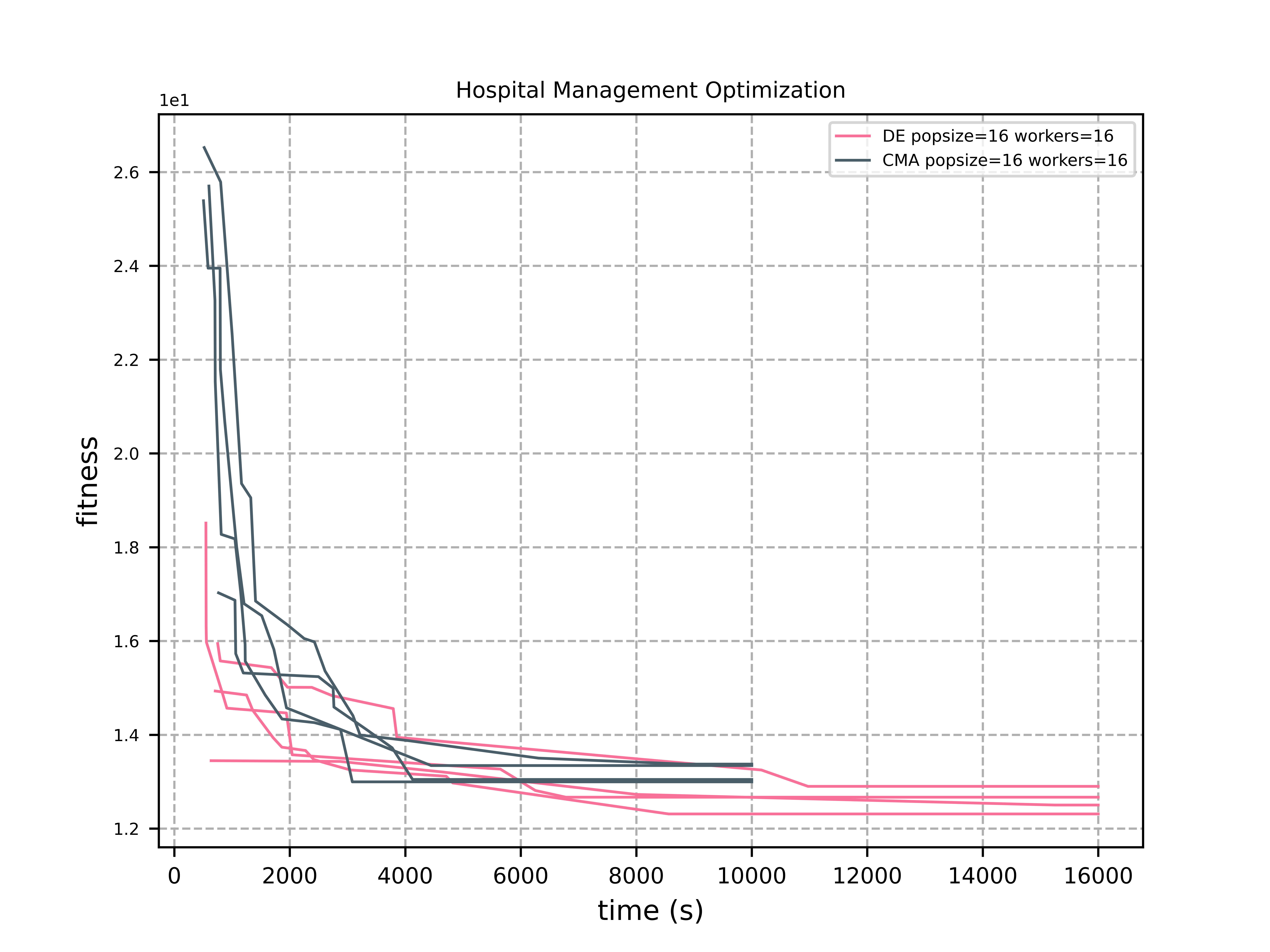
To compare these results with others, we need the number of evaluations achieved by the parallel optimization algorithm, including algorithm overhead: 0.2. So in 1000 seconds, about 200 evaluations can be performed. For comparisons, you therefore need to look at the value in the diagram above at 1000 sec.

Results from the literature

In the literature we found the following results:

Optimisation with a Random ReLU Expansion Surrogate Model

They report the following results for their surrogate-model-based method, which later evolved into MVRSM:

16.29 (+-2.16) and
14.81 (+-0.69) limiting the number of points suggested by the surrogate model

These results are more or less consistent with our DE results after 200 evaluations. Unfortunately, the paper does not state how many runs were executed.

From the paper: "Still, we choose to further fine-tune our approach while disregarding other approaches, and look for ways to reduce the variance"

Unfortunately this will not work, because the variance is caused by the simulation itself. Results vary by about +-2 if you run the simulation multiple times for the same input values. This value increases further for bad input values. For that reason, it is essential to report the number of experiments performed.

Naharro2021

The way results are presented here is even worse. Average and best values for all runs are given, but not the number of experiments performed. Because of the extremely high variation of the simulation results for the same argument vectors, we need the number of experiments to assess the "best result of all runs". That value will definitely improve if the number of runs or evaluations increases. So we should ignore their "best results" and focus on the average values:

DE mean after 750 evaluations: 14.26
DE + DTC mean after 750 evaluations: 14.52
DE + XGBR mean after 750 evaluations: 16.67

They use a Differential Evolution variant with a population size of 8 and a rand/1/exp mutation strategy. Both mutation and recombination factors are set to 0.5. This is very different from fcmaes DE. It is enhanced by blocking candidates using different machine learning classifiers or regressors (DTC, XGBR). This enhancement seems to have a negative effect on the average results. Compare this with our DE average results after 750 evaluations, or 3750 sec, using the diagram above.

Other publications for the hospital management problem present relative results, but no absolute optimization results. Although Jan Hendrik Schön proved that you can almost get a Nobel prize using relative results, see Schön, this makes it difficult to evaluate the tested methods against others.

Exercise: Filtering candidate solutions for DE and MO-DE

Although the results above for filtering DE candidates are discouraging, we created an example that shows how this can be done so you can run your own experiment. The exercise is to adapt the following example, filter.py, which uses a xgboost.XGBRegressor(objective='rank:pairwise') to filter DE or MO-DE candidates for another optimization problem.

Modifying candidate solutions for DE and MO-DE

Recently, explicit support for mixed-integer problems was added to fcmaes DE and MO-DE. One idea behind it is to add random mutations by modifying candidate solutions generated by the algorithm. How can we test this idea for continuous variables? We can do that, but only with the Python variants of the algorithms. de and mode support it, while decpp and modecpp do not yet. We define a method modifier(x) and pass it to the algorithms using the modifier argument:

    def optimizeDE(self):
        self.bestY = 1E99
        self.bestX = []

        def modifier(x):
            dim = len(x)
            min_mutate = 0.5
            max_mutate = max(1.0, dim/20.0)
            to_mutate = np.random.uniform(min_mutate, max_mutate)
            return np.array([x if np.random.random() > to_mutate/dim else
                               np.random.uniform(self.lbs()[i], self.ubs()[i])
                               for i, x in enumerate(x)])

        return de.minimize(self.fun,
            dim = self.dims(),
            bounds = self.bounds(),
            popsize = 24,
            modifier = modifier,
            ints = [v != 'cont' for v in problem.vartype()],
            max_evaluations = 5000,
            workers = 12,
        )

It seems that this modification at least does not harm the results significantly:

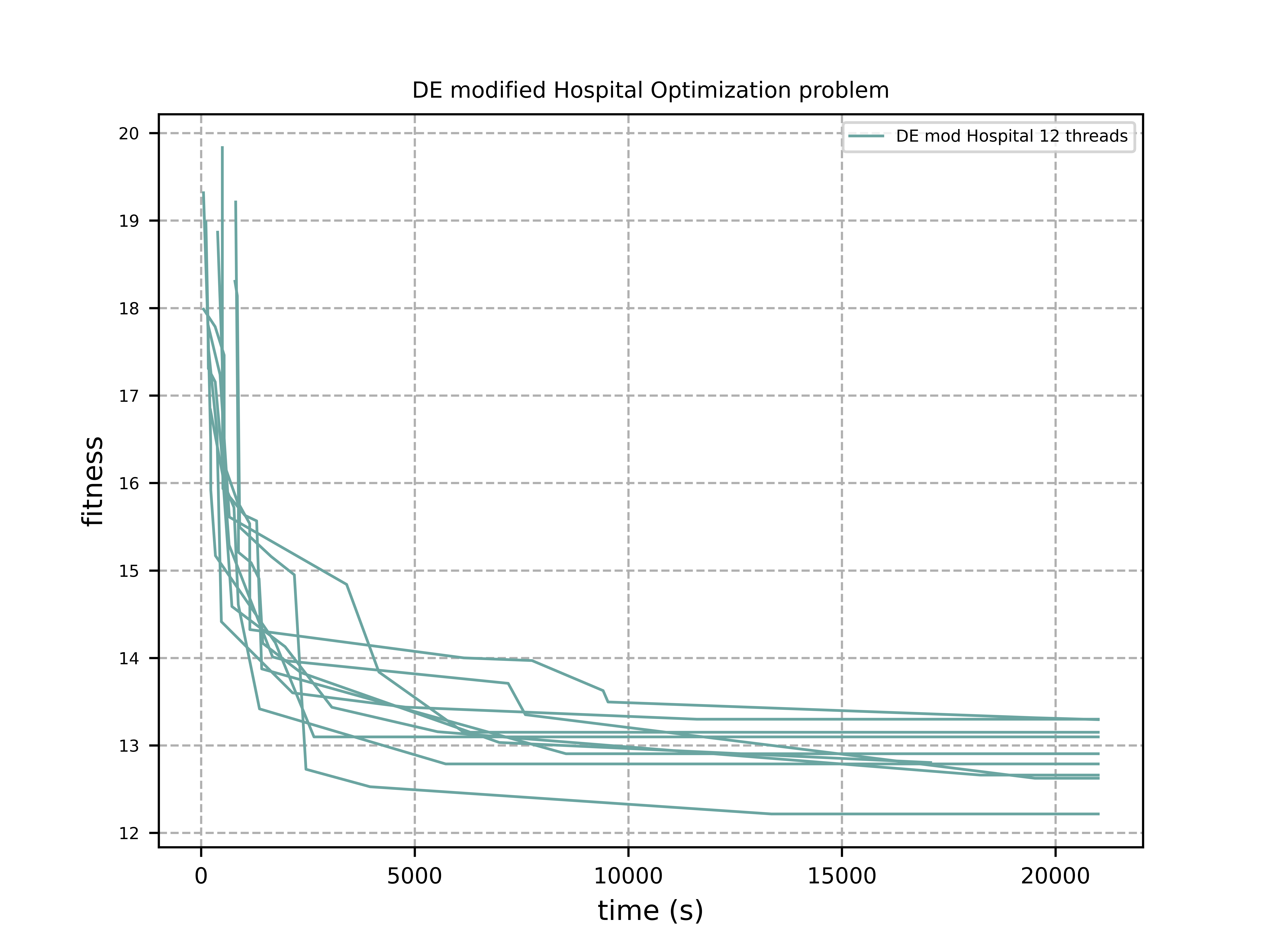
DE modified Hospital Optimization problem

Using only 12 workers instead of 16 increased the number of simulations per second slightly to 0.22. It seems that with 16 parallel simulations our AMD 5950x 16-core CPU is already at its limit. Note that we increased the population size from 16 to 24. Scaling is best when the population size is divisible by the number of workers.

Optimizing the CFD Electrostatic Precipitator problem

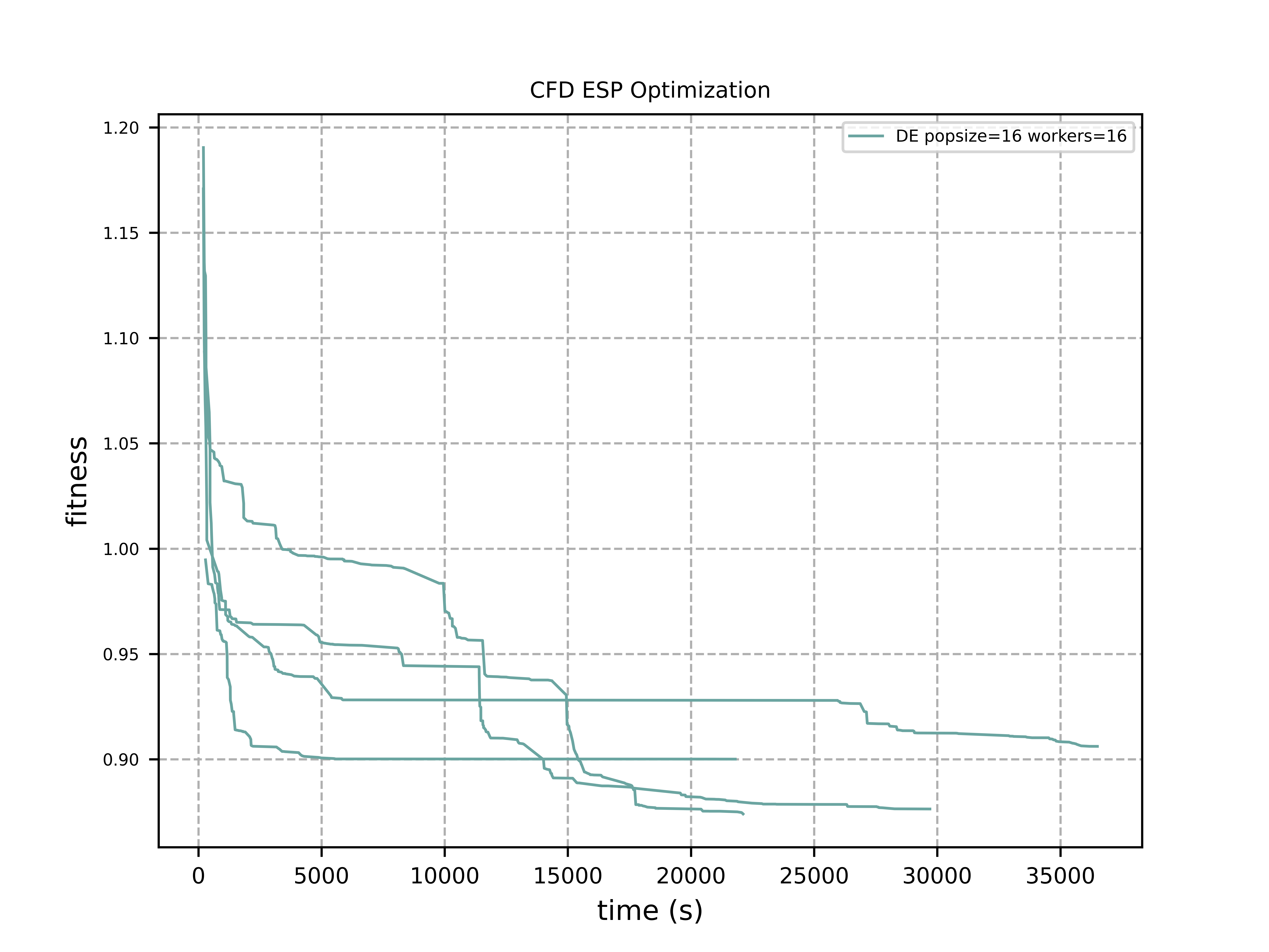
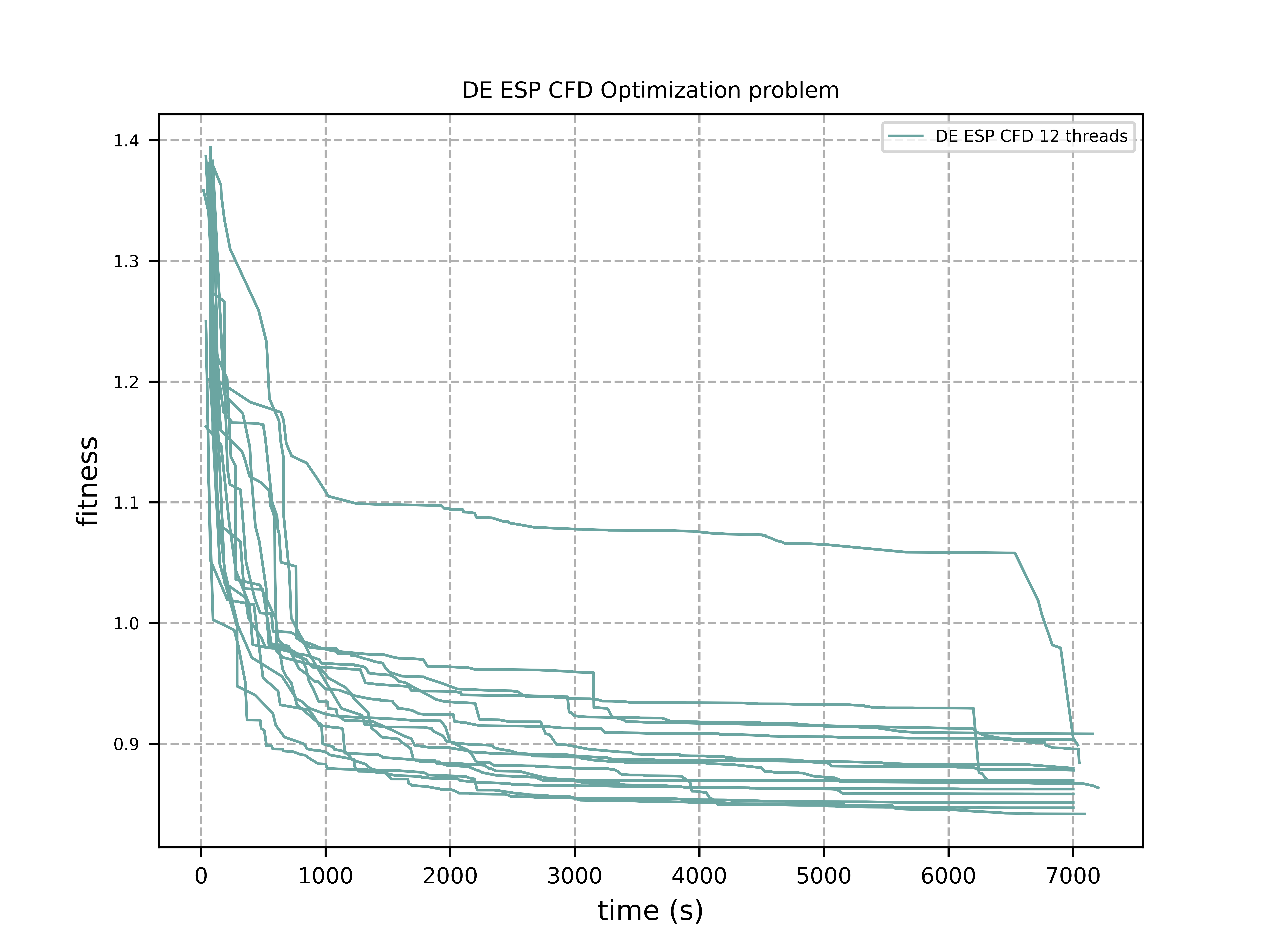
The CFD Electrostatic Precipitator problem can be found at DockerCFDBenchmark.py, see also Electrostatic Precipitator An Electrostatic Precipitator is a large gas filtering installation whose efficiency depends on how well the intake gas is distributed. This installation has slots that can be of various types, each with a different impact on the distribution. This benchmark problem uses the OpenFOAM Computational Fluid Dynamics simulator. The goal is to find a configuration that gives the best resulting distribution.

We executed the "ESP" benchmark with parallel differential evolution:

UPDATE:

After the fcmaes DE algorithm got a mixed-integer upgrade, we ran the experiment again. Since almost all ESP variables are discrete, the result improved significantly:

Parallel execution on an AMD 5950x CPU enabled an execution time of about 1.4 sec / evaluation.

Optimizing a Windmill Wake

A windmill wake simulator based optimization using floris, see Windmill Wake Simulator, code is here: windwake.py The layout of windmills in a wind farm has a noticeable impact on the amount of energy it produces. This benchmark problem uses the FLORIS wake simulator to analyse how much power production is lost when windmills are located in each other’s wake. The objective is to maximize power production.

We executed the WindWakeLayout('example_input.json', n_samples=5) benchmark using example_input.json with parallel differential evolution:

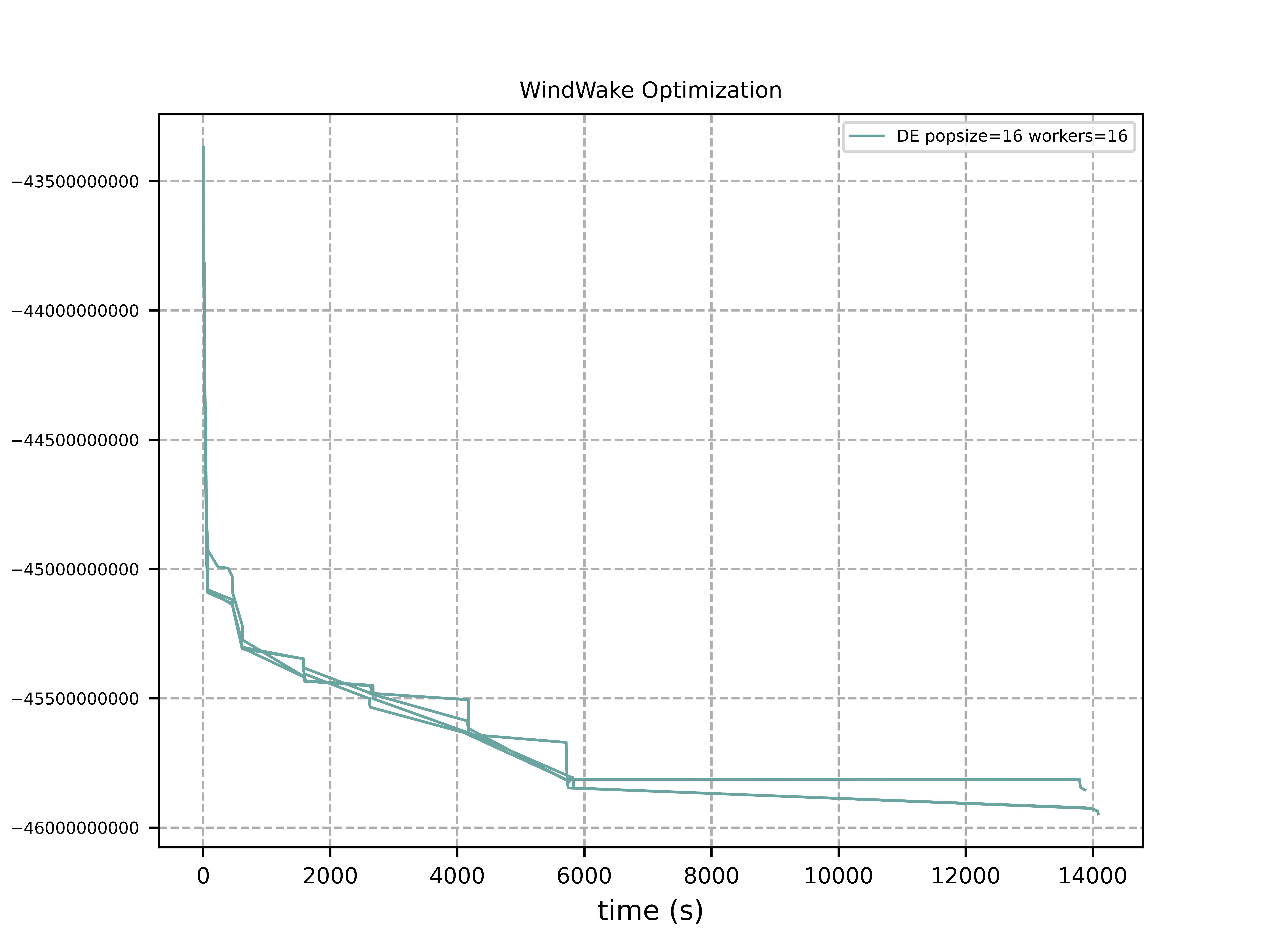
Parallel execution on an AMD 5950x CPU enabled an execution time of about 0.1 sec / evaluation.

Optimizing Hyper-Parameters

Hyper-parameter optimization using xgboost, see HPO / XGBoost, code is here: hpo.py This benchmark uses scikit-learn to build an XGBoost classifier with per-feature preprocessing. Evaluation of a solution is performed by k-fold cross validation, with the goal of maximizing accuracy.

We executed the HPOSFP benchmark using the dataset provided by Semeion, Research Center of Sciences of Communication with parallel differential evolution:

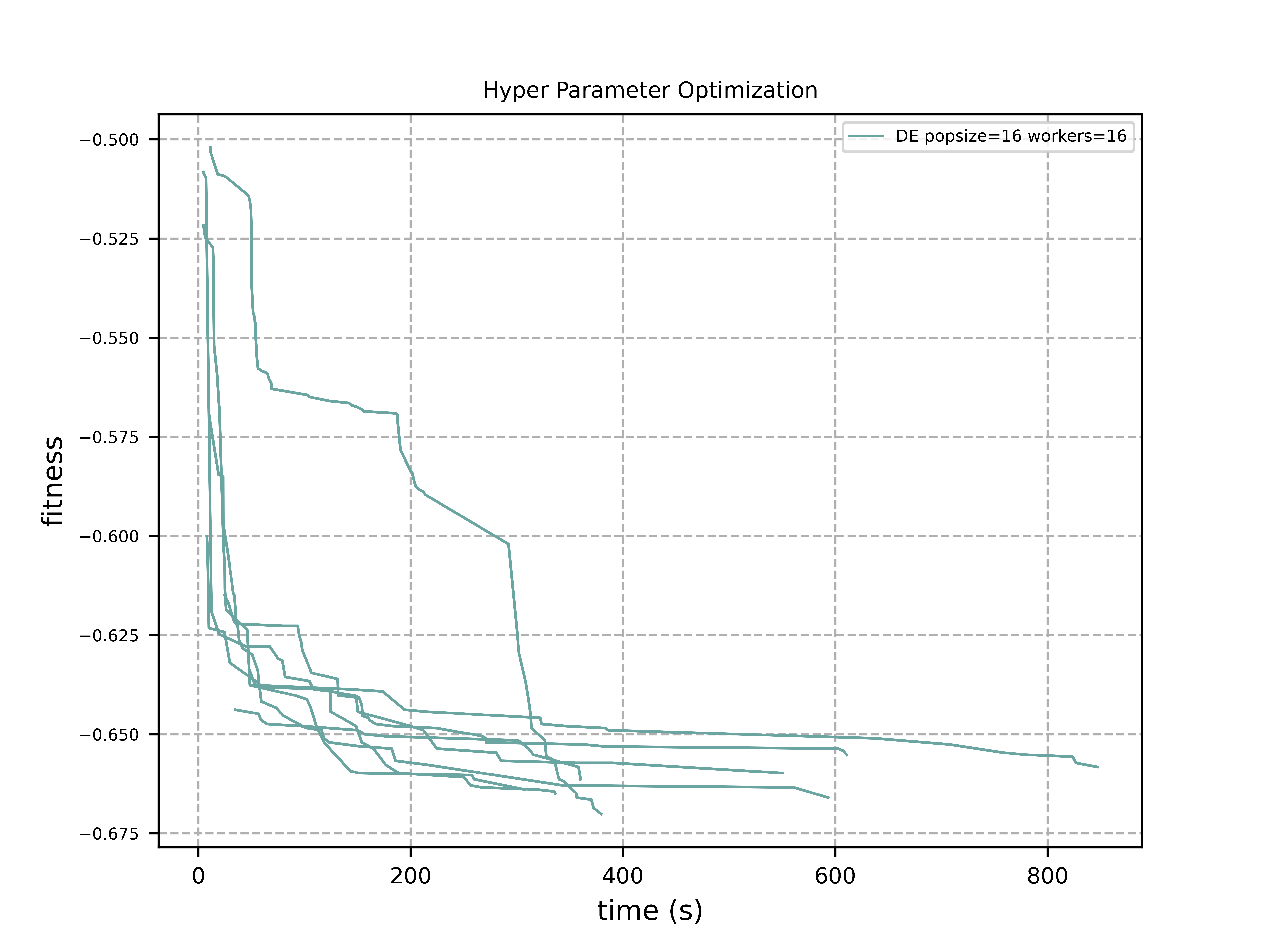
UPDATE:

After the fcmaes DE algorithm got a mixed-integer upgrade, we ran the experiment again. Since many HPO variables are discrete, the result improved:

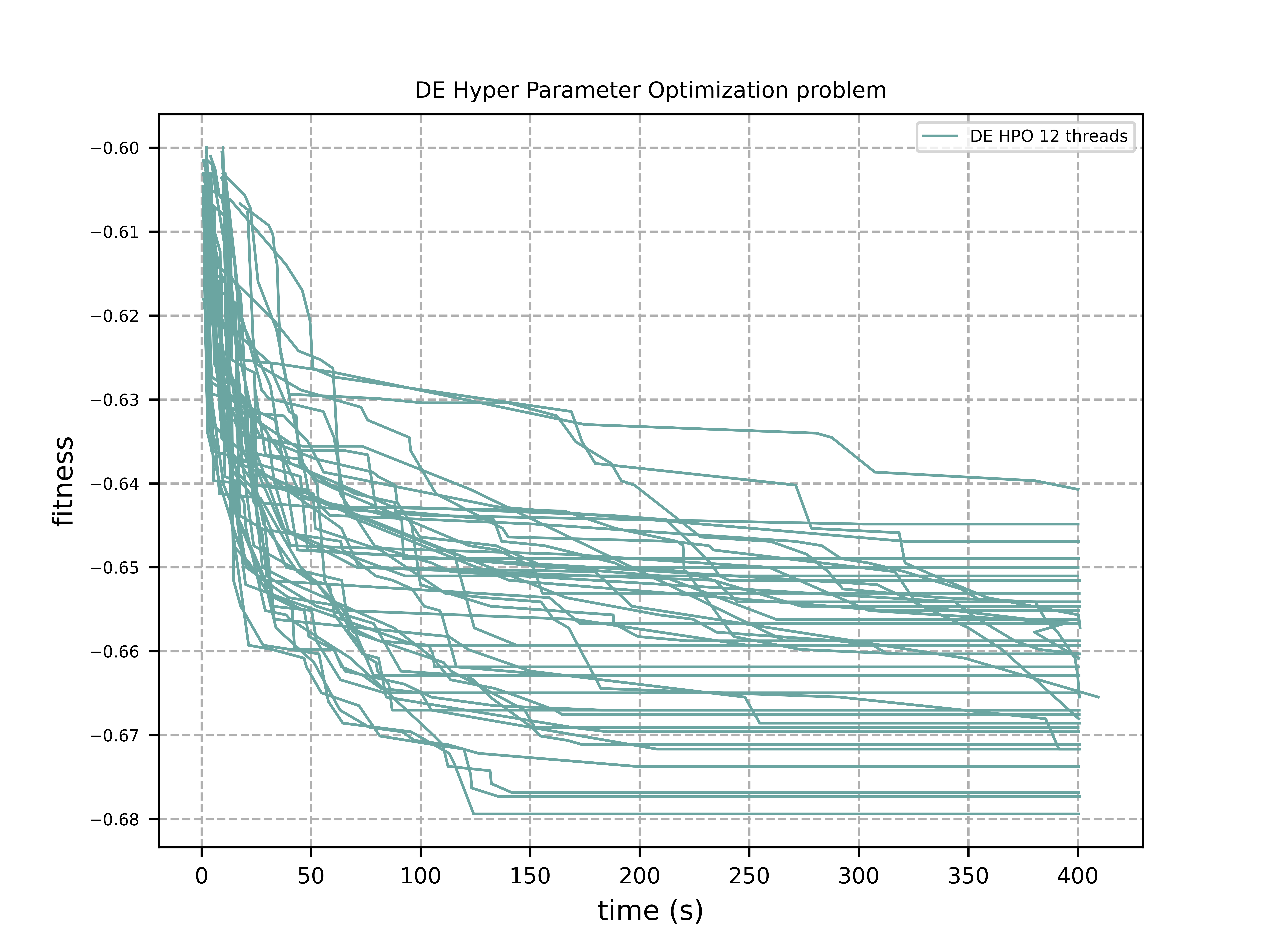
Parallel execution on an AMD 5950x CPU enabled an execution time of about 0.15 sec / evaluation.

In Bliek21 you may find results for surrogate-based optimizers for this problem.