fcmaes - a Python 3 gradient-free optimization library

Modeling Vaccination

This tutorial

Is related to https://github.com/AllenDowney/ModSimPy/blob/master/examples/plague.ipynb from the free book Modeling and Simulation by Allan B. Downey. Unlike the other fcmaes tutorials, the code for this example is licensed under the Creative Commons Attribution-NonCommercial-ShareAlike 4.0 International license, so it cannot be used for commercial purposes. See also Solution Chapter 12.
Shows how to evaluate countermeasures for a disease. How should you distribute a limited budget between them to minimize the infection rate?
Shows how to use multi-objective optimization to produce diagrams of non-dominated solutions that can help plan countermeasures.
Shows how to speed up the simulation using numba.
Shows different ways to visualize multi-dimensional pareto fronts in Python.

The code for this tutorial is here: vaccination.py

Motivation

Modeling and Simulation contains many good ideas for implementing simulations. It uses pandas.Series to represent the time series of a disease outbreak. The example shows, for a fixed overall budget, how different budget splits between two countermeasures

Investing in a hand washing campaign.
Investing in vaccine doses.

affect the final infection rate. It does this by iterating over all possible budget distributions.

But what if the budget is not fixed and you want to explore all possible investment levels? Then the questions become:

How should the money be distributed optimally?
What is the resulting infection rate?

With only two input variables, the two investments, this is still easy to handle with a nested loop and a reasonable step size. But that changes when there are more input variables, more competing objectives, or constraints. It also changes when the solution landscape is rugged and we need a much smaller step size.

For this problem, a multi-objective optimization approach may be overkill. Still, it generalizes well when we add complexity. It can also run simulations in parallel, although that is also possible with a nested loop. In this example, you can think of multi-objective optimization as an "intelligent" nested loop that automatically uses a finer step size near good investment distributions.

Whether we use a nested loop or multi-objective optimization, execution time can become a problem when the simulation is written in Python. We therefore prefer a slightly different way to handle time series, similar to the approach used in our crypto trading tutorial:

Instead of a pandas.Series (one-dimensional), use a pandas.DataFrame. That means we no longer represent the series as a list of objects. Instead, each attribute becomes a separate list stored in a DataFrame column. The main advantage is that we can extract and assign these columns as numpy arrays and pass them to an inner simulator loop implemented with numba. This can speed up the simulation dramatically, which matters when it is called inside a nested loop or a multi-objective optimization. For the vaccination problem we fortunately do not need the full time series at all, because we are only interested in the final infection rate. That computation can easily be delegated to a simulation loop written with numba.

Fast SIR simulation

The disease simulation uses the SIR epidemic model, where SIR stands for

S(t) are those susceptible but not yet infected with the disease.
I(t) is the number of infectious individuals.
R(t) are those individuals who have recovered from the disease and now have immunity to it.

The simulation can be accelerated by several orders of magnitude with numba, as shown below:

    @njit(fastmath=True)
    def fast_update(s, i, r, beta, gamma):
        infected = beta * i * s
        recovered = gamma * i
        return s - infected, i + infected - recovered, r + recovered

    @njit(fastmath=True)
    def fast_simulate(s, i, r, t_end, beta, gamma):
        for t in range(0, t_end):
            s, i, r = fast_update(s, i, r, beta, gamma)
        return s, i, r

fast_simulate replaces sweep_doses from the original example, which fills SRI objects into a pandas.Series. The acceleration may not matter much for this small example, but for larger simulations it is essential that all inner loops run inside numba.

    def sweep_doses(dose_array):
        sweep = SweepSeries()

        for doses in dose_array:
            fraction = doses / num_students
            spending = budget - doses * price_per_dose

            system = make_system(beta, gamma)
            add_immunization(system, fraction)
            add_hand_washing(system, spending)

            results = run_simulation(system, update_func)
            sweep[doses] = calc_total_infected(results, system)

        return sweep

We could also generate the whole series with numba if needed, and store the resulting arrays in a pandas.DataFrame:

    @njit(fastmath=True)
    def fast_simulate(s, i, r, t_end, beta, gamma):
        sa = np.empty(t_end+1)
        ia = np.empty(t_end+1)
        ra = np.empty(t_end+1)
        sa[0] = s
        ia[0] = i
        ra[0] = r
        for t in range(1, t_end+1):
            s, i, r = fast_update(s, i, r, beta, gamma)
            sa[t] = s
            ia[t] = i
            ra[t] = r
        return sa, ia, ra

Objective Fitness Function

How should we define the fitness function that guides the optimization? The result should be a set of non-dominated solutions, a pareto front. It should correspond to the "good" or "interesting" solutions we would otherwise get from a nested loop that iterates first over the vaccination budget and then over hand-washing spending. We are interested in solutions with a low combined budget, so we define the sum budged_doses + spending as one objective and the infection rate infected as the other.

class fcmaes_problem():

    def __init__(self):
        self.dim = 2
        self.bounds = Bounds([0]*self.dim, [budget]*self.dim)

    def simulate(self, budged_doses, spending):
        doses = budged_doses / price_per_dose
        fraction = doses / num_students
        system = make_system(beta, gamma)
        add_immunization(system, fraction)
        add_hand_washing(system, spending)
        results = run_simulation(system, update_func)
        return calc_total_infected(results, system)

    def fitness2(self, x):
        budged_doses = x[0]
        spending = x[1]
        infected = self.simulate(budged_doses, spending)
        return [infected, budged_doses + spending]

    def fitness3(self, x):
        budged_doses = x[0]
        spending = x[1]
        infected = self.simulate(budged_doses, spending)
        return [infected, budged_doses, spending]

problem = fcmaes_problem()

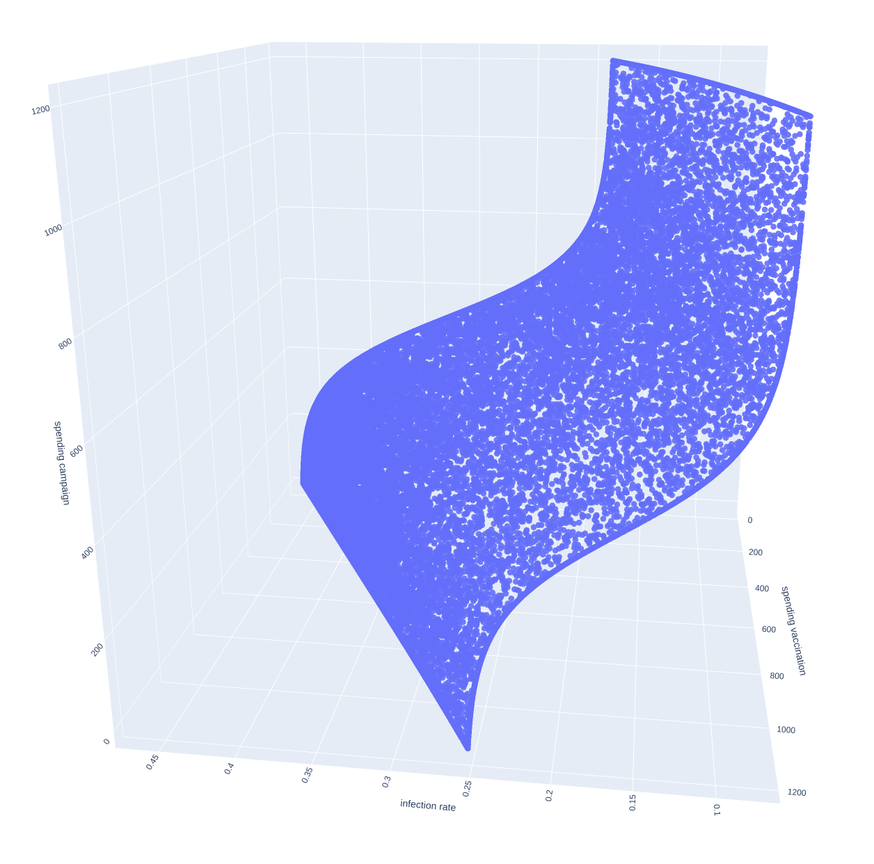
We also define an objective function fitness3 that keeps both budgets separate. This lets us create a 3-dimensional chart that shows how all budget distributions relate to the resulting infection rate.

Compute the 2-objective Pareto Front

fcmaes offers two different parallelization modes:

Parallel function evaluation

In this mode, a single optimization evaluates the fitness function in parallel. The advantage is faster convergence. You need fewer evaluations to produce a good set of non-dominated solutions, the pareto front.

    xs, ys = mode.minimize(mode.wrapper(problem.fitness2, 3, interval=1000), 3,
               problem.ncon, problem.bounds,
               popsize = 256, max_evaluations = 25600, nsga_update=False,
               workers=8)

Result

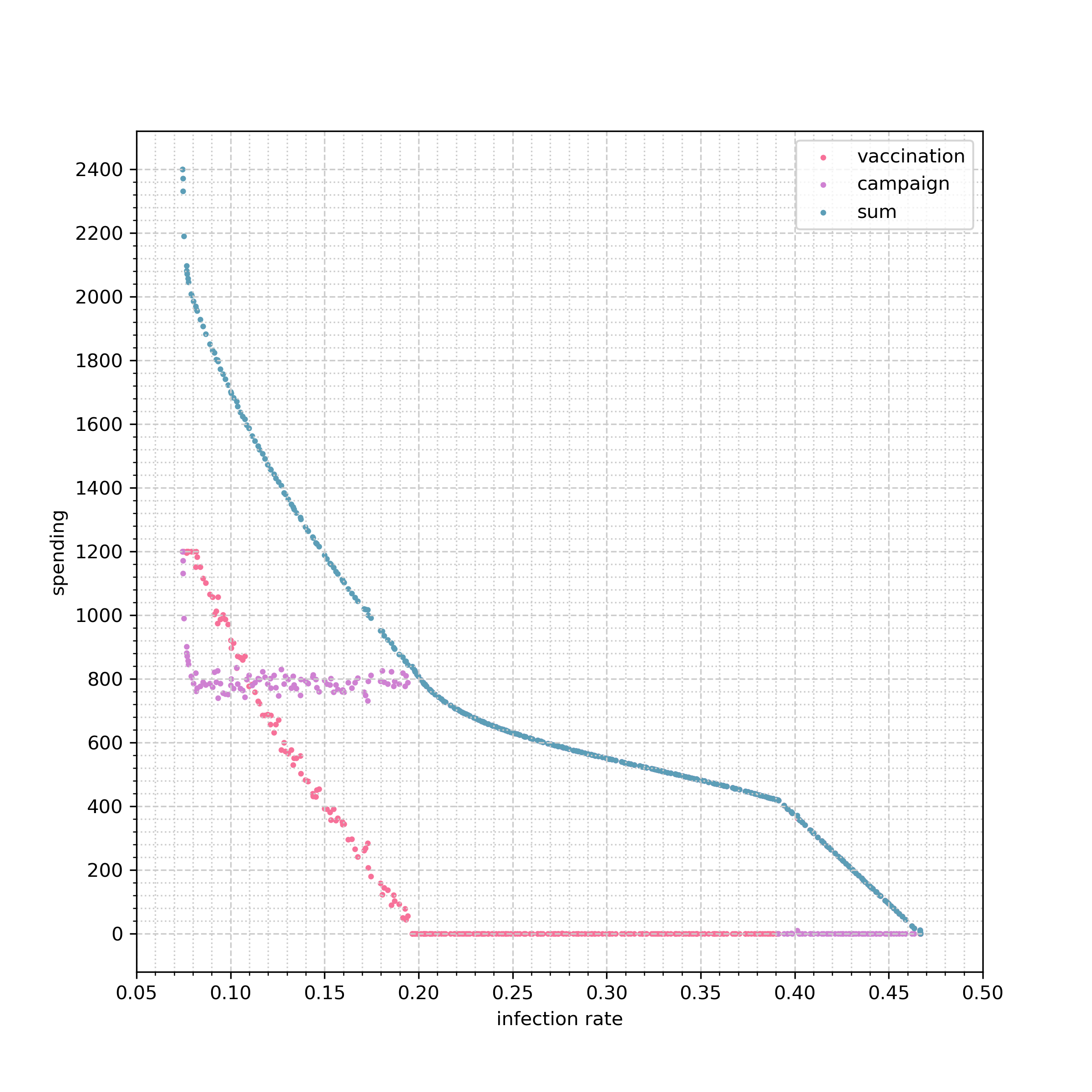
Only 8 workers are used because the parallelization overhead is high. More workers would not improve the evaluation rate further. If the fitness evaluation is more expensive, it dominates the parallelization overhead and this problem disappears. Because of our numba-based tuning we get about 1450 evaluations/sec using parallel function evaluation, and about 6800 evaluations/sec using parallel optimization on a 16 core / 32 thread AMD 5950 CPU. The whole optimization produces a 512 solution pareto front in about 17 seconds for parallel function evaluation (25000 evaluations) and a 7573 solution pareto front in about 83 seconds (561000 evaluations)

For comparison, the original non-numba simulation performs 277 simulations / sec using parallel function evaluation, and about 286 evaluations/sec using parallel optimization. In that case you need to set workers=32 for mode.minimize to fully utilize the CPU, because the parallelization overhead is now smaller compared to the cost of a function evaluation.

In single-threaded mode, the original non-numba simulation performs only 13.3 simulations / sec. The numba-optimized version reaches about 450.

So the speed gain factors are as follows:

Table 1. Simulation speed gain factors
parallelization	original	numba
none	1.0	33.8
parallel function	20.8	109.0
parallel optimization	21.5	511.2

So the maximum speedup on the AMD 5950 CPU 16 core CPU was 511: parallel optimization / numba simulation compared to single-threaded / original simulation. For larger and more serious simulations or optimizations, this kind of speedup matters.

Parallel optimization

In this mode, the whole optimization is performed in parallel. The advantage is better scaling and more evaluations per second. The disadvantage is slower convergence, so you need more evaluations. But you also get more solutions in the pareto front:

    xs, ys = modecpp.retry(mode.wrapper(problem.fitness2, 2, interval=1000), 2,
               0, problem.bounds, popsize = 128, max_evaluations = 12800,
               nsga_update=False, num_retries = 64, workers=32)
    moretry.plot("pandemy", 0, xs, ys)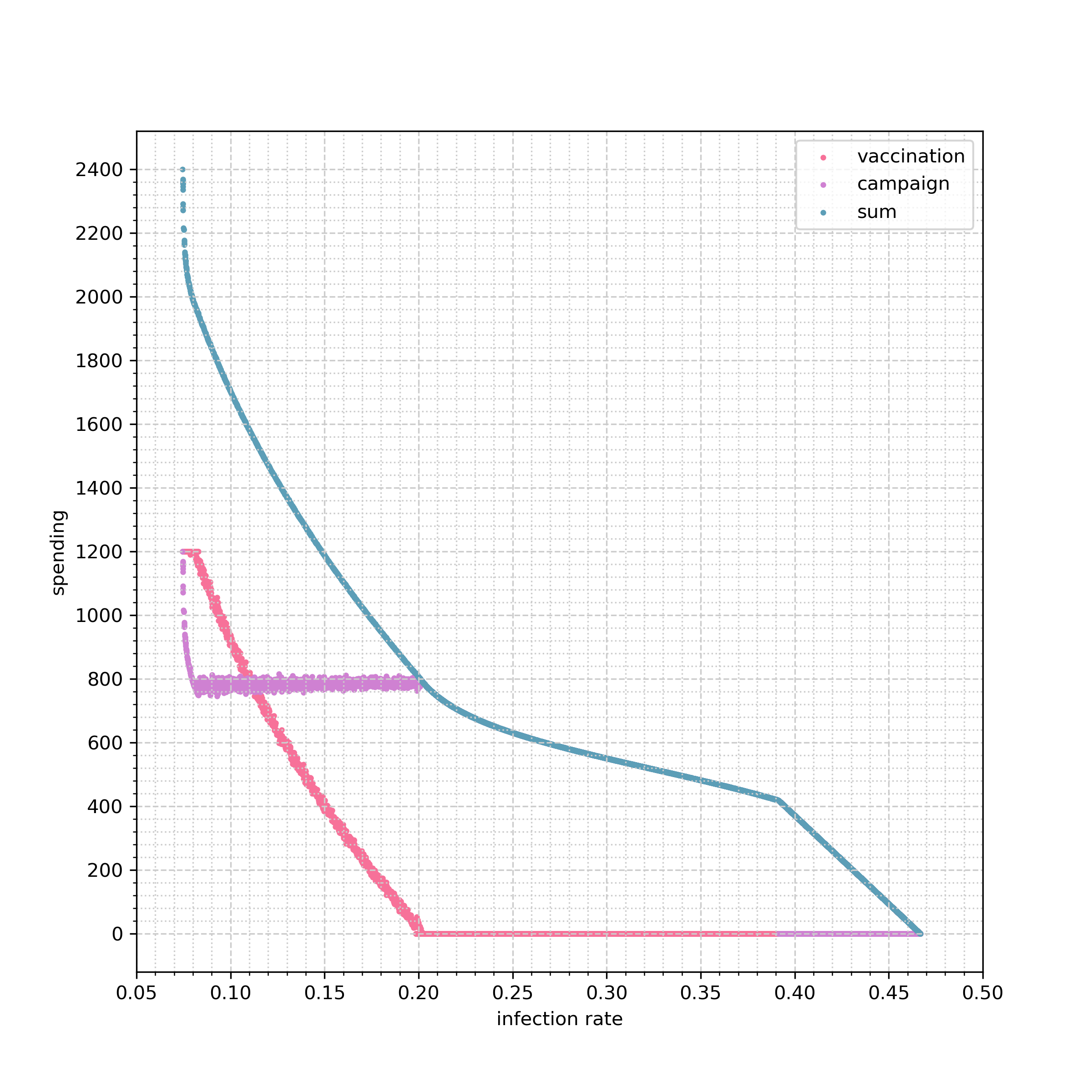

Interpretation of the result

Parallel optimization gives a more detailed picture because the better scaling lets us compute a larger solution set.

We see that:

We should not invest more than 800 for the hand-washing campaign, since for a final infection rate < 0.20 only more money invested in vaccination helps.
As long as we invest 800 for the hand-washing campaign, each increase of the vaccination budget further reduces the final infection rate significantly.
If our overall budget is between 400-800, all the money should go to the hand-washing campaign.
If it is less than 400, all the money should be invested in vaccination.

Did you expect this result? I was surprised.

Compute the 3-objective Pareto Front

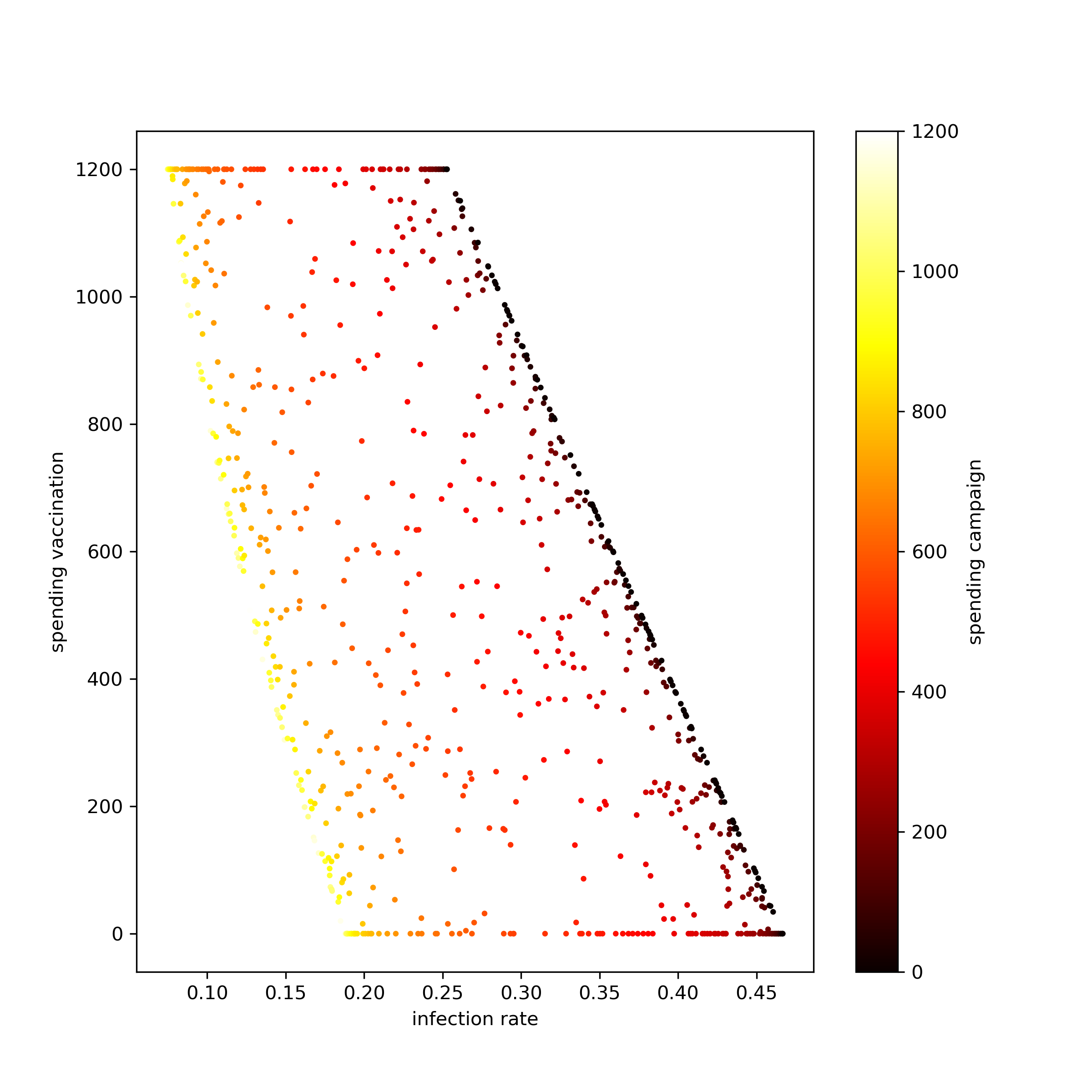
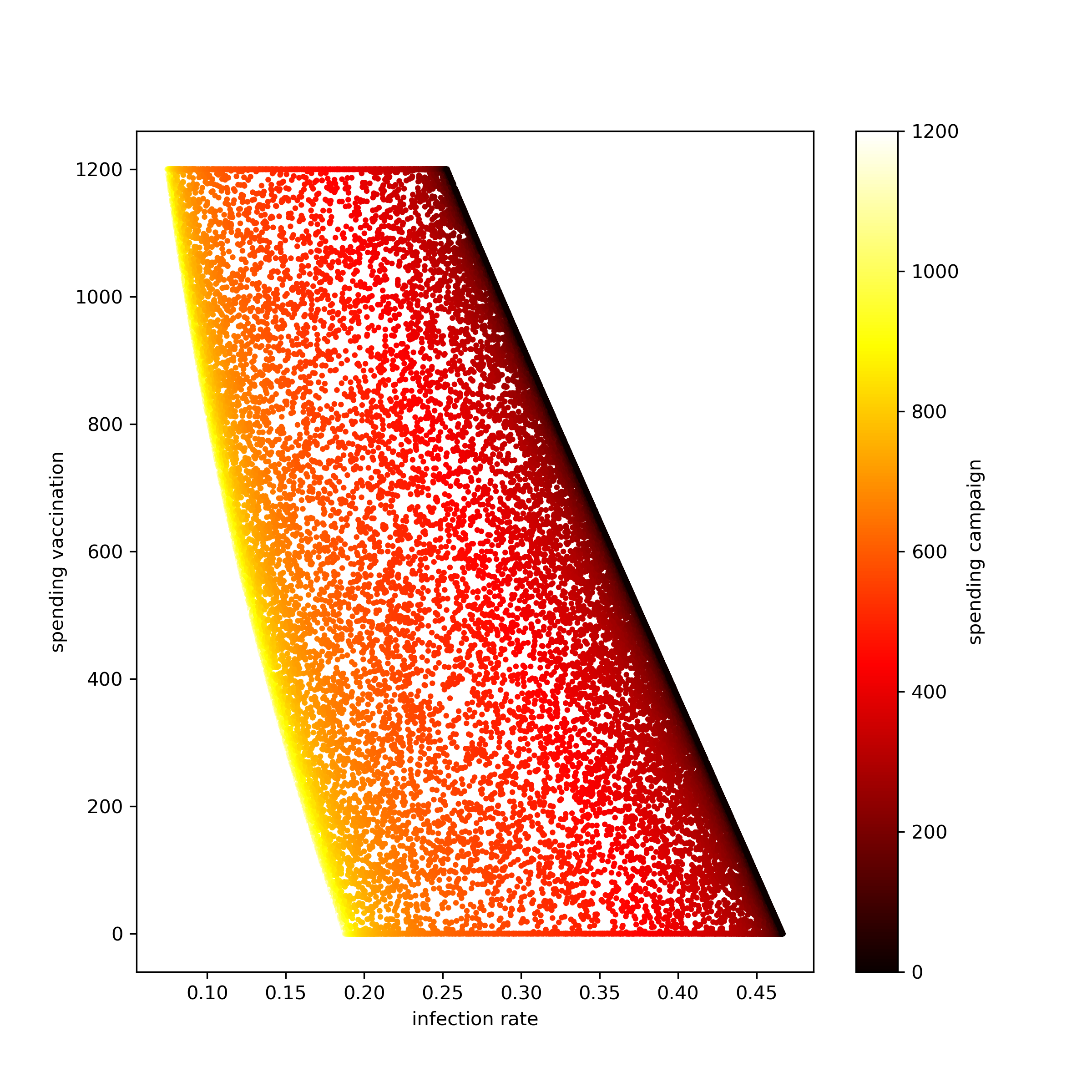
We use the same algorithms again, this time with the 3-objective variant fitness3. Performance is very similar to the 2d variant, but now we can see how both campaign spending and vaccination budget influence the final infection rate.

Parallel function evaluation

    xs, ys = mode.minimize(mode.wrapper(problem.fitness3, 3, interval=1000), 3,
                0, problem.bounds, popsize = 512, max_evaluations = 25600,
                nsga_update=False, workers=8)
    plot3d(xs, ys, task)

Result

This time we produce two pictures. One uses a heatmap to represent the third dimension:

The other uses a 3d perspective:

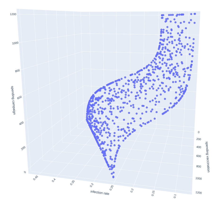
When you run the example, you will notice that you can interact with the picture in the browser. This is important because it makes the 3d result much easier to understand.

Parallel optimization

    xs, ys = modecpp.retry(mode.wrapper(problem.fitness3, 3, interval=1000), 3,
                0, problem.bounds, popsize = 256, max_evaluations = 25600,
                nsga_update=False, workers=32)
    plot3d(xs, ys, task)

Again we get a more detailed picture with parallel optimization because the better scaling lets us compute a larger solution this way. Note that this is not the case for expensive objective functions, because then both methods scale similarly.

Exercise

Is the result dependent on the optimization library used? To answer this question, try nevergrad, a very popular optimization library (> 40000 downloads last month, see https://pypistats.org/packages/nevergrad ). You may start with NGOpt, CMA, DE, or TwoPointsDE, but be warned: finding a nevergrad multi-objective algorithm that is able to reproduce the result above is challenging. You may try something like:

    import nevergrad as ng
    fit = mode.wrapper(problem.fitness2, 2, interval=1000)
    instrum = ng.p.Instrumentation(
            ng.p.Array(shape=(problem.dim,)).set_bounds(problem.bounds.lb, problem.bounds.ub))
    optimizer = ng.optimizers.TwoPointsDE(parametrization=instrum, budget=5000, num_workers=8)
    optimizer.minimize(fit, verbosity=0)
    front = optimizer.pareto_front()
    xs = np.array([p.value[0][0] for p in front])
    ys = np.array([p.losses for p in front])
    plot2d(xs, ys, "TwoPointsDE")

If you do not succeed, try pymoo. This exercise shows that when numba speeds up the fitness function, the optimization algorithm overhead becomes relevant. nevergrad is not designed for fast fitness functions.

Conclusion

fcmaes multi-objective optimization can replace a nested loop that enumerates all solutions produced by a simulation.
Advantages for this kind of application are
- Automatic parallelization.
- Automatic adjustment of the step size.
Visualization of multi-dimensional solution landscapes can assist the decision-making process.
If the solution landscape is rugged, or if there are many dimensions, objectives, or constraints, a nested loop will no longer work.
For larger and more serious simulations or optimizations, it matters that parallelization and numba together can achieve a speed factor > 500.