fcmaes - a Python 3 gradient-free optimization library

Solving a complex scheduling problem using continuous optimization

Can Python and continuous optimization solve a difficult scheduling problem efficiently? Can they stay competitive when other teams use hand-tuned code, strong heuristics, and a lot of hardware?

Many people would answer "no" for three reasons:

Python is slow, especially when the objective function contains loops.
Continuous optimization is hard to parallelize well across the many cores of a modern CPU. scipy does not support this.
Standard algorithms from scipy do not work well when discrete arguments are encoded as continuous values and then converted to integers. Even more advanced methods such as Differential Evolution do not converge fast enough.

With a single-threaded optimization algorithm, the objective function used here reaches only about 1.8 evaluations per second, even on a modern AMD 5950 CPU.

But consider the following:

We can scale by about 16x by using all cores of a modern 16 core CPU such as the AMD 5950.
We can speed up the objective function by about 450x with Numba, for a combined speedup of roughly 7200x when parallelization is included.
We can use continuous optimization algorithms that handle discretized inputs much better.

Whether that is enough to beat carefully tuned genetic algorithms coded in C/C++ is still open. This tutorial makes a narrower point: C++ does not win automatically.

Important concepts used

Indirect encoding

We need a decoder to map the parameter encoding, given as a vector of continuous variables, to an actual schedule. The decoder also handles the problem constraints and guarantees that the solution is valid. This idea is well established in the literature.

Indirect objective

The optimizer does not see the real objective directly. Instead, it sees a specific objective, or several objectives in the multi-objective case, that were designed to guide the search. This is familiar from weighted sums for constraint handling. Using multi-objective optimization for a single-objective problem is less common. It does not work equally well for all problems, but this scheduling problem is a good fit.

Update

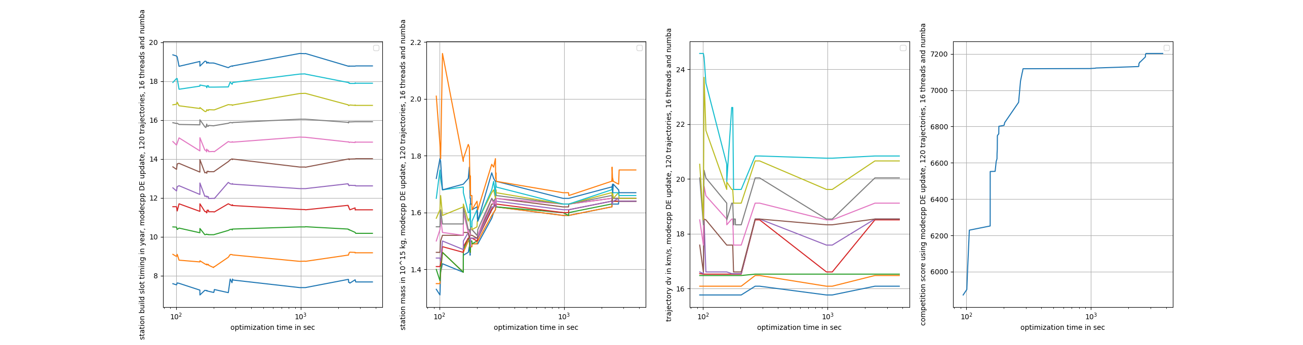
After applying a similar approach to the more general multi-objective flexible jobshop problem, see JobShop, we observed an unexpected result: the new multi-objective algorithm MoDe produced excellent single-objective results. We therefore extended this tutorial with the same idea. The outcome was even more surprising: score 7203 with 120 trajectories to choose from.

GTOC 11

GTOC is an international competition on global trajectory optimization. The 11th competition, GTOC11, ended in November 2021. Of the 92 participating teams, only a small fraction managed to upload a valid solution in time:

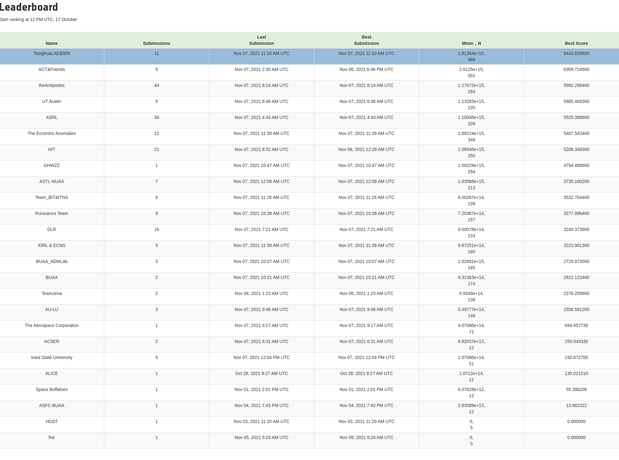
This tutorial is aimed at the other teams. It shows how to handle the "hard part" of the problem efficiently. The full problem description is available in the problem statement.

The task is to start building a Dyson sphere by constructing a ring of 12 stations, equally spaced on a circular orbit around the sun. Whole asteroids are used as building material and are transferred in one piece to the sphere. Ten motherships start from Earth. Each one visits an asteroid sequence chosen from a huge set of 83453 asteroids and leaves an attenuator there. The attenuator uses asteroid mass to generate constant continuous thrust and move the asteroid to one of the 12 Dyson stations.

Only one station can be built at a time, and there must be a 90 day wait before the next station can be built. Dyson sphere station construction and the mothership start times are both restricted to a 20 year window (video).

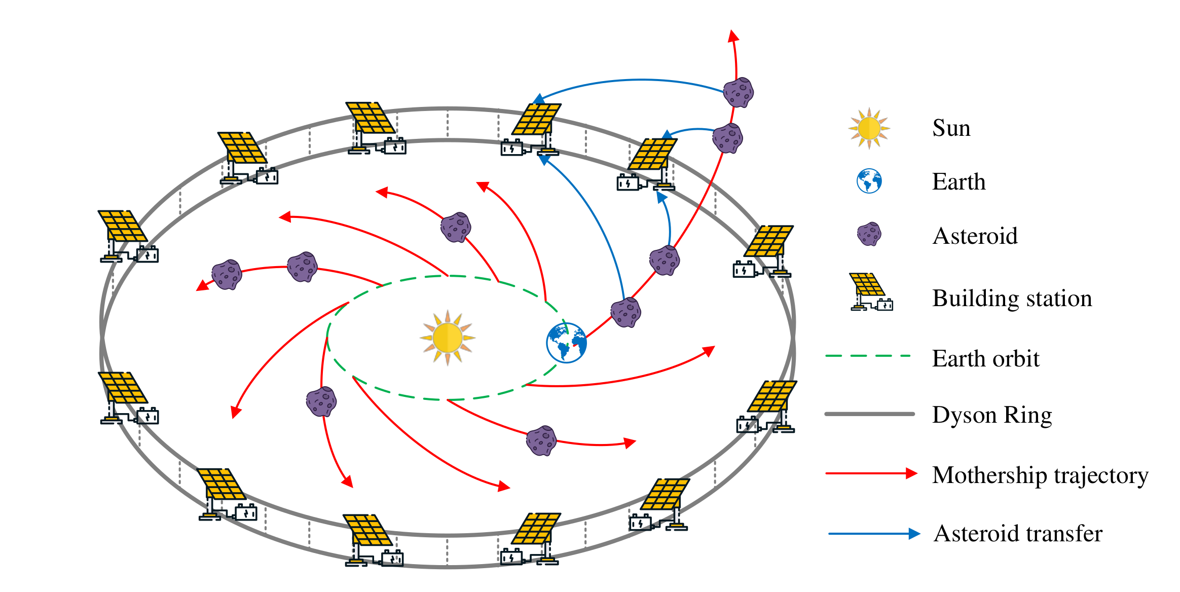
Propellant, represented by the magnitude of the mothership delta velocity impulses, is not limited, but it reduces the competition score. After a mothership visits an asteroid, that asteroid must be transferred to a Dyson sphere station using a continuous-thrust maneuver with fixed acceleration magnitude. Each asteroid has a specific mass. Part of that mass is consumed to power the transfer, so the arrival mass depends on both the original mass and the transfer time.

The goal is to maximize and balance the mass delivered to all stations. The competition score depends on two quantities:

the remaining asteroid mass arriving at the least-supplied station, which should be maximized
the total delta velocity of the motherships, which should be minimized

Most parts of the task are straightforward for astrophysicists:

Selection of a suitable Dyson sphere
Estimation of the maximal asteroid arrival mass at the Dyson sphere, independent from phasing
Estimation of the asteroid arrival mass at the Dyson sphere for a given station and transfer timing
Computation of good mother ship trajectories visiting asteroids with high estimated remaining mass at the Dyson sphere

The hard part is the combination step. We must choose the order and arrival time windows for the Dyson stations, decide which ten mothership trajectories to take from a much larger set of strong candidates, and assign asteroid transfers so that the score is maximized.

Additional aspects,

Inclination and size of the Dyson ring
Initial phasing of the Dyson ring stations

are not part of the optimization shown here. We leave them out so that we can precompute a table of good mothership trajectories together with a set of optimal asteroid transfers. That avoids expensive calculations during optimization. The tradeoff is that the full table has to be regenerated for each different Dyson ring, so the table design matters.

In this tutorial we treat that table as given and focus on the optimization itself. The table used here was produced by "Team Jena", which ranked only 16th in the competition, so it is far from optimal. We used both Tsinhuas and ESAs submitted Dyson spheres so that we could compare our method with the results achieved by these teams. The same objective function is used for all results.

Below we look at the effect of three factors:

Selection of the optimization algorithm
Usage of Numba
Utilization of parallel multi threaded optimization

Asteroid transfer table

For each asteroid visited by any mothership trajectory, we compute a set of transfers together with the mothership arrival times. These define the time windows available for the asteroid transfers. For each sphere revolution, for each sphere station, and for each asteroid start time window, we can compute the optimal asteroid transfer that minimizes time of flight for the fixed continuous thrust.

This produces a table in which each row lists:

asteroid id
trajectory index
station number
asteroid mass
delta velocity to reach the asteroid from the previous one
start time
transfer time

The remaining asteroid mass at the sphere station can be derived from the asteroid mass and the transfer time. The table used in this tutorial contains about 163.000 asteroid transfer opportunities for the 50 best trajectories found.

For a valid row selection representing 10 mothership trajectories and one transfer for each visited asteroid, we can compute the estimated score from the sum of the trajectory delta velocities and the sum of the remaining asteroid masses arriving at each Dyson station.

The asteroid transfer data is stored as a compressed CSV file and read as a pandas data frame.

DataFrame:
         asteroid   station  trajectory  ...   dv       transfer_start  transfer_time
0          73418        1          31  ...  3.500261        2.816957       2.891577
1          73418        2          31  ...  3.500261        2.738180       2.852998
2          73418        3          31  ...  3.500261        2.599462       2.843404
3          73418        4          31  ...  3.500261        2.464159       2.827190
4          73418        5          31  ...  3.500261        2.335112       2.807543
...          ...      ...         ...  ...       ...             ...            ...
162611     68957        5          29  ...  0.403024       16.836162       2.456525
162612     68957        6          29  ...  0.403024       16.676695       2.486187
162613     68957        7          29  ...  0.403024       16.511622       2.556778
162614     68957        8          29  ...  0.403024       16.376856       2.644360
162615     68957       12          29  ...  0.403024       16.918...

[162615 rows x 7 columns]

You can replace this table with your own and check which score the algorithm computes for your solution.

Implementation

The complete implementation is available at scheduling.py. It is heavily commented and should be easy to adapt to a different scheduling problem. The code was tested on Linux with the Anaconda Python environment. On Windows, use the Linux subsystem for Windows if possible, because Python multithreading has issues there. Do not forget to run pip install fcmaes --upgrade to get the newest fcmaes version.

Design of the argument vector

The approach stays simple because we only need an efficient objective function that computes the estimated score for an argument vector containing:

10 trajectory indices selecting the trajectories for the 10 motherships
12 station indices defining the build order of the stations
11 values representing the limits of the build time slots. These are sorted and multiplied by 20 years, the full mission time

To simplify the comparison of results, we use ESAs Dyson sphere with a = 1.32AU, but we had to perform our own search and approximation of possible asteroid transfers. If we restrict ourselves to the best 10 trajectories and therefore disable trajectory selection during optimization, as ESA did during the competition, we reproduce ESAs competition score and mass distribution almost exactly. This indicates that our optimization is not inferior even when trajectories are fixed. If we let the optimization choose the 10 trajectories, the score improves by about 400, but it still does not reach Tsinhua or winner territory. A smaller Dyson sphere is probably needed to improve further.

The bounds are chosen to avoid rounding errors when the continuous argument values are converted to integer indices.

We use a special parallelization algorithm with smart boundary management (SBM). It returns the best argument vectors and function values. For this problem, it works best in combination with a DE→CMA optimization sequence. The optimization log can be used to monitor progress.

    transfers = pd.read_csv('data/' + name + '.xz', sep=' ', usecols=[1,2,3,4,5,6,7], compression='xz',
                    names=['asteroid', 'station', 'trajectory', 'mass', 'dv', 'transfer_start', 'transfer_time'])
     ...
    # bounds for the objective function
    dim = 10+2*STATION_NUM-1
    lower_bound = np.zeros(dim)
    # lower_bound[10+STATION_NUM:dim] = 0.00001
    upper_bound = np.zeros(dim)
    lower_bound[:] = 0.0000001
    upper_bound[10:] = 0.9999999
    upper_bound[:10] = TRAJECTORY_NUM-0.00001 # trajectory indices
    bounds = Bounds(lower_bound, upper_bound)

    # smart boundary management (SMB) with DE->CMA
    store = advretry.Store(fitness(transfers), bounds, num_retries=10000, max_eval_fac=5.0, logger=logger())
    advretry.retry(store, de_cma(10000).minimize)

Alternatively, the fcmaes parallel retry mechanism can be used with BiteOpt or other optimization algorithms.

    store = retry.Store(fitness(transfers), bounds, logger=logger())
    # apply BiteOpt algorithm in parallel
    retry.retry(store, Bite_cpp(1000000, M=6).minimize, num_retries=320)

Smart boundary management gives a better final score, but it can be slower if it is configured poorly for this task.

Design of the objective function

We implement the objective function as a Python function class. call defines the function itself, while the object stores the context, namely all data frame columns as NumPy arrays.

class fitness(object):

    def __init__(self, transfers):
        ...
        self.asteroid = transfers["asteroid"].to_numpy()
        self.station = transfers["station"].to_numpy()
        self.trajectory = transfers["trajectory"].to_numpy()
        self.transfer_start = transfers["transfer_start"].to_numpy()
        self.transfer_time = transfers["transfer_time"].to_numpy()
        self.mass = transfers["mass"].to_numpy()
        self.dv = transfers["dv"].to_numpy()

We precompute and store the sum of the delta velocities for all trajectories.

        self.trajectory_dv = trajectory_dv(self.asteroid, self.trajectory, self.dv)

The objective function calls select. This function chooses the asteroid transfers represented by the argument vector, computes the used mass, adds the corresponding delta velocities of the selected branches, and returns the score:

   def __call__(self, x):
        # determine the minimal station mass
        min_mass, slot_mass = select(self.asteroid, self.station, self.trajectory, self.mass,
                        self.transfer_start, self.transfer_time, x)
        sdv = select_dvs(self.trajectory_dv, x)
        return -score(min_mass, sdv)

For each row we check the following:

Is the corresponding trajectory selected, and is the targeted station correct? The arrival time determines the time slot and therefore the station number assigned to that slot.
Has the asteroid already been visited before? Two trajectories may contain the same asteroid, so we greedily keep the transfer with the larger remaining asteroid mass.
Then we accumulate the masses transferred to each station.

Execution time for select is reduced dramatically by Numba, a JIT compiler that accelerates functions annotated with @njit. select uses nested loops. In plain Python that would be a bad idea, but with Numba it works well.

@njit(fastmath=True)
def select(asteroid, station, trajectory, mass, transfer_start, transfer_time, x):
    ...
   for i in range(asteroid.size):
        tr = int(trajectory[i]) # current trajectory
        if trajectories[tr] == 0: # trajectory not selected
            continue
        ast_id = int(asteroid[i]) # asteroid transferred
        stat = int(station[i]) # dyson sphere station targeted
        m = mass[i] # estimated asteroid mass at arrival time
        time_of_flight = transfer_time[i] # TOF of asteroid transfer
        arrival_time = transfer_start[i] + transfer_time[i] # arrival time of asteroid transfer
        # which station time slot ?
        for slot in range(STATION_NUM):
            max_time = times[slot+1] # time interval of time slot
            slot_time = times[slot]
            min_time = slot_time + WAIT_TIME # we have to wait 90 days
            if min_time >= MAX_TIME:
                continue
            if arrival_time >= slot_time and arrival_time <= max_time: # inside time slot
                if stat == stations[slot]: # does the station fit?
                    tof = time_of_flight
                    #if we have to fly a non optimal transfer, arrival mass is reduced
                    if arrival_time < min_time: # 90 DAYS are not yet over
                        to_add = min_time - arrival_time # add time difference
                        to_add *= math.sqrt(1 + to_add/WAIT_TIME) # add some more time to enable transfer
                        tof += to_add
                    mval = (1.0 - YEAR*tof*ALPHA) * m # estimated asteroid mass at arrival time
                    if ast_val[ast_id] > 0: # asteroid already transferred
                        old_slot = int(ast_slot[ast_id])
                        min_mass = np.amin(slot_mass) # greedily replace if current mass is higher
                        old_mass = slot_mass[old_slot] # but never replace at a nearly minimal slot
                        if (old_slot == slot or min_mass < 0.99*old_mass) and ast_val[ast_id] < mval:
                            # replace with actual transfer, remove old asteroid mass
                            slot_mass[old_slot] -= ast_val[ast_id]
                        else: # keep old transfer, don't use the new one
                            mval = 0
                    if mval > 0:  # register actual transfer
                        slot_mass[slot] += mval
                        ast_val[ast_id] = mval
                        ast_slot[ast_id] = slot
    ...

Instead of using only the minimal station mass, we also include the other station masses with weights that decay exponentially by mass rank. This helps early in the search, when the minimal mass is often 0. The score shown in the output is still computed only from the minimal mass.

    slot_mass.sort()
    min_mass = slot_mass[0]
    f = 1.0
    for m in slot_mass:
        min_mass += f*m
        f *= 0.5
    return min_mass, slot_mass

Both the station order and the selected branches must be disjoint. For the branches, we use a utility function that converts a continuous input vector s into a disjoint integer vector:

@njit(fastmath=True)
def next_free(used, p):
    while used[p]:
        p = (p + 1) % used.size
    used[p] = True
    return p

@njit(fastmath=True)
def disjoined(s, n):
    disjoined_s = np.zeros(s.size, dtype=numba.int32)
    used = np.zeros(n, dtype=numba.boolean)
    for i in range(s.size):
        disjoined_s[i] = next_free(used, s[i])
    return disjoined_s, used

For the station order, we use numpy.argsort:

@njit(fastmath=True)
def dyson_stations(x, n):
    stations = np.argsort(x[10:10+n])
    # station numbers start with 1
    return np.array([s+1 for s in stations])

Hints

This section collects a few practical hints for readers who still struggle with the "easy" parts of the task.

Selection of a suitable Dyson sphere

Determine the average inclination of all "heavy" asteroids with limited eccentricity.
Choose Dyson spheres with this inclination and different semimajor axis a with 1.0AU < a < 1.6AU.
Estimate the maximal arrival mass at the Dyson sphere for all "heavy" asteroids and choose the sphere with the largest average arrival mass divided by a, since the score is proportional to the minimal station mass divided by a.

The Dyson sphere can later be fine tuned while good mother ship trajectories are being computed. These trajectories can then be reevaluated for different Dyson spheres to maximize the estimated score.

Finding good mothership trajectories

This can be done with beam search and a branch selection criterion based on time / delta velocity / estimated maximal remaining asteroid mass, using different weights to maximize trajectory diversity. A small search breadth, about 1000 branches, combined with a huge number of searches (> 100000), increases the chance of finding many good trajectories with disjoint asteroid visits. Use a precomputed grid of asteroid positions and linear approximation to speed up trajectory expansion during search.

What you should not do:

Use the same set of asteroids visited first at depth 1 of the search for all runs. Use a random selection instead.
Favor a specific weight for the sum of the delta velocity for all search runs. Let the search decide by using random weights instead.
Exclude a large fraction of asteroids from the search. I excluded only the worst 23000 because I observed worse results otherwise.

Estimation of the arrival mass

You could learn from Tsinhua, the winners, or from ESA, who developed a machine learning approach that estimates the final mass more reliably. A simple and fast alternative is to divide the transfer into n equal time windows, or segments, and replace the continuous thrust by n impulses, also called deep space maneuvers (DSMs), applied at the center of these segments. This is the Sims-Flanagan method. As n increases, accuracy improves, but so does the computational effort.

With four segments, we need only 8 input variables: 6 for the two 3-dimensional impulses dv_1 and dv_4, plus 2 for start and arrival time. dv_2 and dv_3 can be derived using the Lambert algorithm. The impulses must be limited according to the fixed continuous thrust constraint, and the objective is minimal time of flight. Differential evolution with retry and different random initial values works very well here.

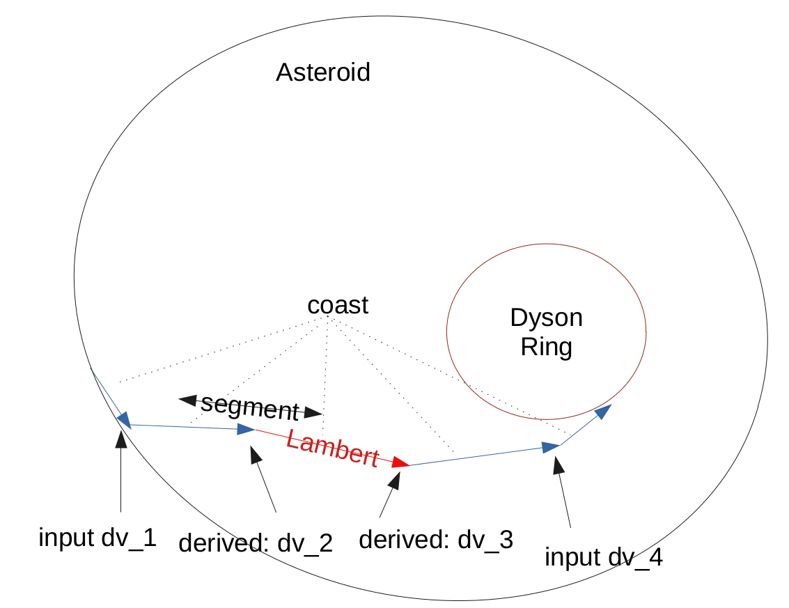
You can either compute specific transfers to each station for different time windows to build the input table for the scheduling algorithm, or you can treat the station as an additional discrete argument without time limits and compute an estimated maximal remaining mass at the station. The second option is useful when evaluating trajectories during search.

Optimal delta velocity

During the conference after the GTOC11 competition, Dario Izzo from the ESA&friends team asked which delta velocity should be targeted for the trajectories.

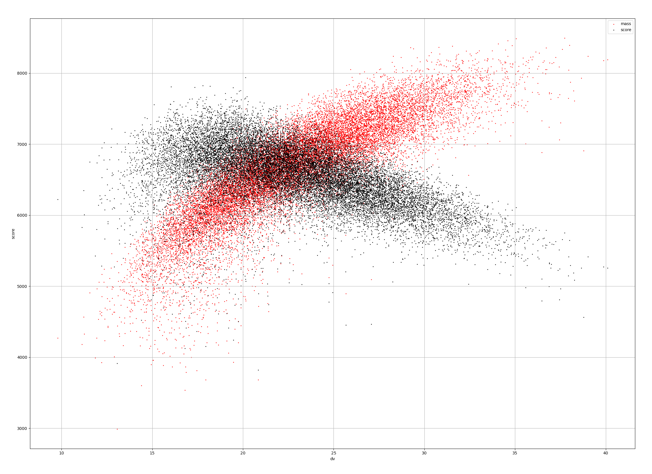
The plot shows the delta velocities of about 20.000 good trajectories. Each point represents the best trajectory found in a search-breadth=1000 run with random roots and random weights. The potential collected mass increases with delta velocity, but the corresponding score does not. We compute the score by taking the sum of the trajectory asteroid masses as the minimal mass and the sum of the trajectory delta velocities for all ten motherships. This is roughly an upper bound on the score that a scheduling algorithm can achieve.

QD update

Recently QD algorithms were added to fcmaes. They are a good fit for answering Dario Izzo’s question about the optimal delta velocity. We first define a QD fitness function that returns the score together with a "behavior vector" d used to enforce diversity. Here we simply use the minimal mass and delta velocity.

   def qd_fun(self, x): # quality diversity
        _, slot_mass = select(self.asteroid, self.station, self.trajectory, self.mass,
                        self.transfer_start, self.transfer_time, x)
        sdv = select_dvs(self.trajectory_dv, x)
        _, dv_val = score_vals(np.amin(slot_mass), sdv)
        sc = score(np.amin(slot_mass), sdv)
        y = -sc
        self.evals.value += 1
        d = np.array([np.amin(slot_mass)*1E-15, dv_val])
        return y, d

We then apply the fcmaes diversifier QD meta-algorithm and plot the resulting QD archive, which represents a diverse set of solutions for different minimal mass and delta velocity values:

def nd_optimize():
    problem = get_fitness()
    problem.qd_dim = 2
    problem.qd_bounds = Bounds([1.0,15],[2.2,24])
    niche_num = 10000
    name = "scheduler_nd"
    opt_params0 = {'solver':'elites', 'popsize':200}
    opt_params1 = {'solver':'BITE_CPP', 'max_evals':1000000, 'stall_criterion':3}
    archive = diversifier.minimize(
         mapelites.wrapper(problem.qd_fun, 2, interval=100000, save_interval=200000000),
         problem.bounds, problem.qd_bounds,
         workers = 32, opt_params=[opt_params0, opt_params1],
         max_evals=100000000, archive = None,
         niche_num = niche_num, samples_per_niche = 20)
    print('final archive:', archive.info())
    archive.save(name)

We configure the algorithm to use CVT-Map-Elites in parallel together with a BiteOpt improvement emitter. This produces:

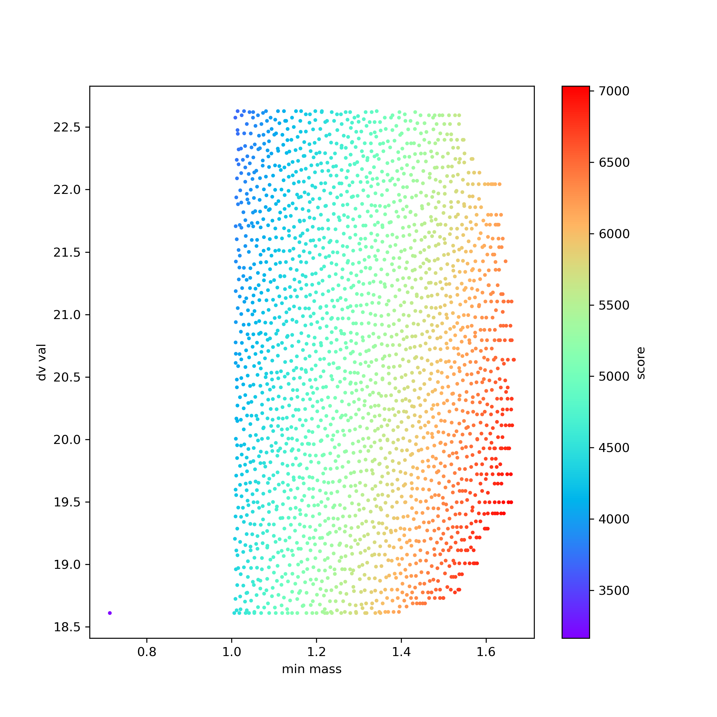
The quality of a solution is indicated by its color. There are no dark red solutions, near and above score 7000, below delta velocity values of 19. It seems that some delta velocity is needed to increase the minimal asteroid mass arriving at the Dyson station.

The complete code is available at scheduling.py.

How to use this algorithm to produce a GTOC11 solution

The scheduling algorithm shown here is only one part of a full GTOC11 solution. It turns a huge set of approximated asteroid transfers, associated with a number of good mothership trajectories, into a much smaller transfer selection associated with only 10 trajectories while maximizing the approximated score. With the table used in this example, it reduces 321264 transfers to about 390 transfers.

Converting an approximated transfer into a real continuous-thrust transfer that passes the GTOC11 validation is CPU intensive. The scheduling algorithm helps by reducing the number of transfers that need this expensive conversion:

Apply the scheduling algorithm for a limited time to determine which transfers need to be converted.
After conversion, adapt the transfer timing in the table.
Repeat this process until no time slot violations occur.

In later iterations, only the transfers that are still approximated need to be converted.

As a final step, we can exploit the fact that only the station with the least mass matters for the score. Some transfers can probably be removed without reducing the minimal mass, which may lower the sum of delta velocities required for the corresponding mothership trajectory.

Update

After applying a similar approach to the more general multi-objective flexible jobshop problem, see JobShop, we observed another unexpected result: the new multi-objective algorithm MoDe produced excellent single-objective results. GTOC11 is also, at its core, a multi-objective problem with two objectives:

Minimize the delta velocities of the mothership trajectories
Maximize the minimal Dyson station mass

The competition score combines these through a non-linear formula. As a competition participant, you do not really need a Pareto front. You need a single strong solution. But a multi-objective algorithm may still produce a better single-objective result. It also provides a set of alternative high-scoring solutions, which is useful because the results are still approximations and later need to be converted into continuous-thrust trajectories.

To test this idea, we need a multi-objective variant of the fitness function. We simply add a method fun to the fitness class:

@njit(fastmath=True)
class fitness(object): # the objective function
...
    def fun(self, x):
        min_mass, slot_mass = select(self.asteroid, self.station, self.trajectory, self.mass,
                        self.transfer_start, self.transfer_time, x)
        sdv = select_dvs(self.trajectory_dv, x)
        scr, dv_val = score_vals(np.amin(slot_mass), sdv)
        y = -scr
        ys = [-min_mass*1E-10, dv_val]
        ...
        if y < self.best_y.value:
               self.best_y.value = y
    return ys

We still track improvements of the single-objective score, but we hide that from the optimizer. From the optimizer’s point of view, the target is the two-objective vector [-min_mass*1E-10, dv_val].

As multi-objective optimizer we use MoDe, implemented in C++. We call it through the parallel retry mechanism:

    # multi objective optimization 'modecpp' multi threaded, NSGA-II population update
    xs, front = modecpp.retry(fit.fun, fit.nobj, fit.ncon, fit.bounds, num_retries=640, popsize = 96,
                max_evaluations = 3000000, nsga_update = True, logger = logger(), workers=16)

MoDe offers two population update mechanisms: one derived from NSGA-II and one from DE. Even when the NSGA-II population update is used, the algorithm differs significantly from standard NSGA-II. There is no tournament selection, and MoDe can handle constraints. In contrast to the flexible job shop problem, the DE population update also works well here. The NSGA-II update improves faster at first, but the DE update often gives better final results. With DE population update, you can declare the first 10 variables, the trajectory selection, as integer variables via the ints parameter:

    # mixed integer multi objective optimization 'modecpp' multi threaded, DE population update
    fit.bounds.lb[:10] = 0
    fit.bounds.ub[:10] = TRAJECTORY_NUM-1 # integer variables include upper bound
    xs, front = modecpp.retry(fit.fun, fit.nobj, fit.ncon, fit.bounds, num_retries=640, popsize = 128,
                max_evaluations = 10000000, nsga_update = False, logger = logger(), workers=16,
                ints=[True]*10+[False]*(dim-10))

With a larger evaluation budget and population size, the DE population update found a score of 7197 after one hour using 60 trajectories:

evals = 56562254: time = 3604.9 s = 7197 a = 385 t = [7.28, 8.75, 10.33, 11.12, 12.42, 13.59, 14.74, 15.9, 16.68, 17.86, 19.08] s = [12, 1, 2, 3, 4, 5, 6, 9, 8, 11, 7, 10] b = [19, 50, 4, 43, 36, 45, 54, 29, 55, 49] m = [1.67, 1.68, 1.68, 1.68, 1.68, 1.68, 1.68, 1.69, 1.71, 1.73, 1.74, 1.84] dv = [21.84, 20.04, 19.74, 19.5, 18.26, 19.12, 16.53, 19.9, 16.09, 22.18]

A score of 7329 was reached with 120 trajectories to choose from:

evals = 39043304: time = 3067.0 s = 7329 a = 385 t = [7.15, 8.84, 10.14, 11.46, 12.47, 13.74, 14.72, 15.66, 16.6, 17.91, 19.12] s = [9, 1, 11, 10, 5, 8, 2, 4, 3, 12, 6, 7] b = [104, 70, 55, 117, 12, 66, 89, 106, 54, 34] m = [1.65, 1.65, 1.66, 1.66, 1.66, 1.66, 1.66, 1.67, 1.67, 1.69, 1.69, 1.69] dv = [15.77, 18.33, 16.09, 18.54, 20.66, 18.51, 19.62, 16.61, 16.53, 21.77]

You can customize the termination criteria by providing an is_terminate callback:

    xs, front = modecpp.retry(fit.fun, fit.nobj, fit.ncon, fit.bounds, num_retries=640, popsize = 96,
                  max_evaluations = 3000000, nsga_update = True, logger = logger(),
                  is_terminate = is_terminate(), workers=16)
   ...

   class is_terminate(object):

    def __init__(self):
        self.count = 0
        self.score = 0

    def __call__(self, x, y):
        self.count += 1
        score = - y[0] / (A_DYSON * A_DYSON * y[1])
        if self.score < score:
            self.score = score
        if self.count == 300000 and self.score < 20500:
            logger().info("fail: " + str(self.score))
            self.score = 0
            self.count = 0
            return True
        else:
            return False # don't terminate optimization

Here we check whether the "virtual" score reaches "20500" after 300000 function calls in the current thread. Note that the first component of the objective vector is based on a mass value that includes more than just the minimal mass, because that helps the optimization process.

Detailed results

For the results below, we mainly used a transfer table based on Tsinhuas 1.1 AU dyson sphere.

Number of trajectories offered for selection

During the competition, many teams did not integrate trajectory selection into their asteroid transfer and station selection optimization. Instead, they fixed a set of 10 good trajectories and repeated the optimization for different sets. Is that a good idea?

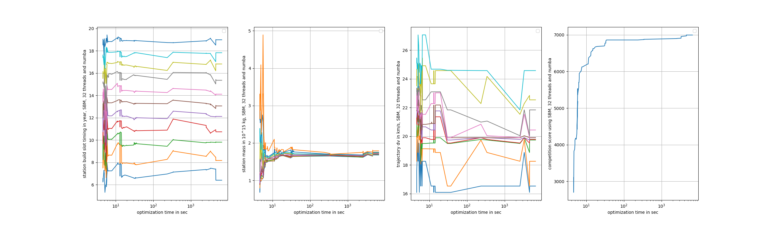
If you have about 60 promising trajectory candidates, then there are 75394027566 possible combinations (n choose k calculator). To test this, we preselected the best 10, 60, and 120 trajectories from a set of 3000 good trajectories obtained from 20000 beam search runs. With 60 trajectories we get a score of about 7000:

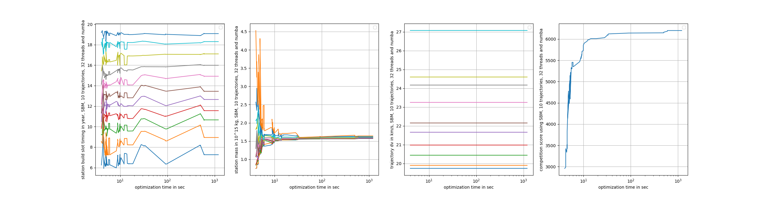
Restricting the choice to the best 10 reduces the score to about 6200:

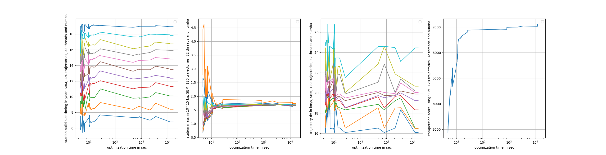
With 120 trajectories we can improve to about 7100:

These results show:

Integrating trajectory selection directly into the optimization objective works very well.
The 10 additional variables increase the problem dimension, but they do not slow down the optimization significantly.

Note that we have not included the 120-trajectory transfer file because of its size, but you can reproduce the first two results.

Update

The pattern is similar with the multi-objective modecpp optimizer: score 7067 for 60 trajectories and score 7201 for 120 trajectories.

Size of the Dyson sphere

The average Dyson sphere size chosen by the teams was a = 1.2 AU. The two top teams, Tsinhua and ESA, chose opposite ends of the range: Tsinhua used a = 1.1 AU, ESA used a = 1.32 AU. We used Tsinhuas sphere to compute our transfer table. What happens if we instead use ESAs larger sphere while keeping exactly the same method and optimization approach? The result is surprising:

We end up with a score of about 6600, only 500 less than for the Tsinhuas sphere. The real competition results differ by about 2200. It may be that the longer transfers allow more room for improvement if you work very hard to minimize time of flight. We did not adapt the search to the different spheres. Only the trajectory ordering depended on the transfers found.

Comparison of algorithms for scheduling

The results below can be summarized in a few points:

Continuous optimization works for mixed-integer problems such as scheduling.
The 450x objective-function speedup from Numba is essential if you want reasonable results.
Parallel optimization and multithreading improve performance significantly.
The best method is Smart Boundary Management + DE→CMA. SBM was originally developed for GTOP (see smart-retry for its performance on those problems). It also works very well for GTOC11 scheduling when configured appropriately. Like PAGMOs archipelagos, SBM uses communication between threads and therefore cannot be run in a single-threaded setup.
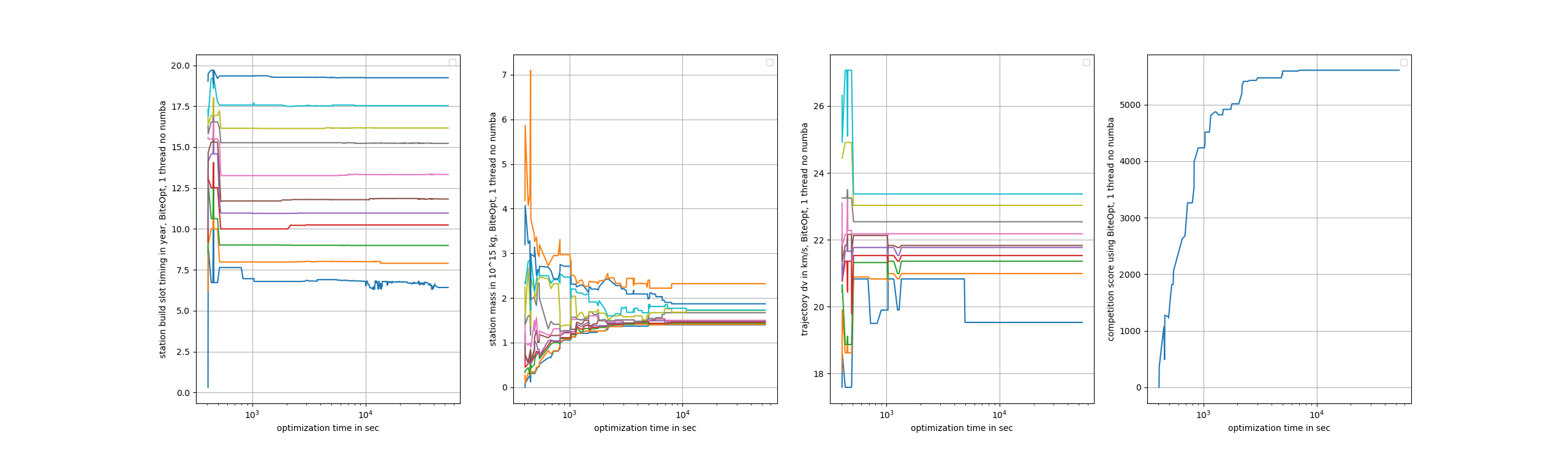
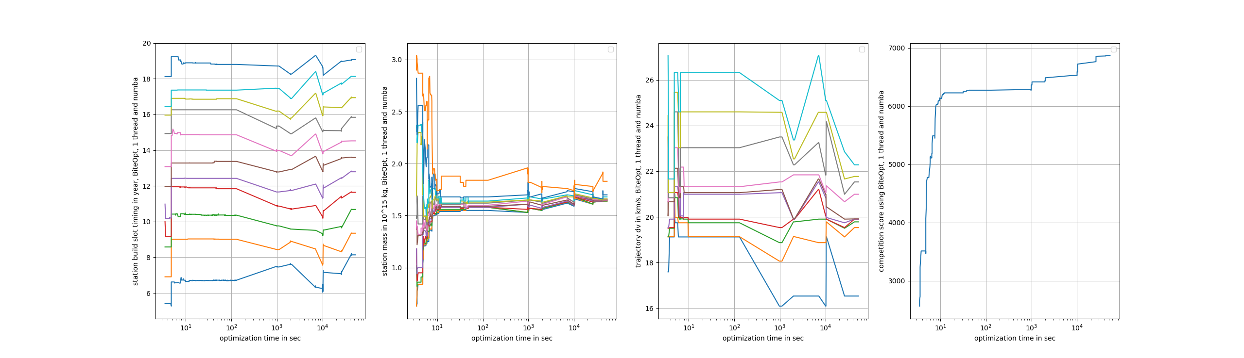
The best single-threaded algorithms are BiteOpt and the fcmaes implementation of CMA-ES.
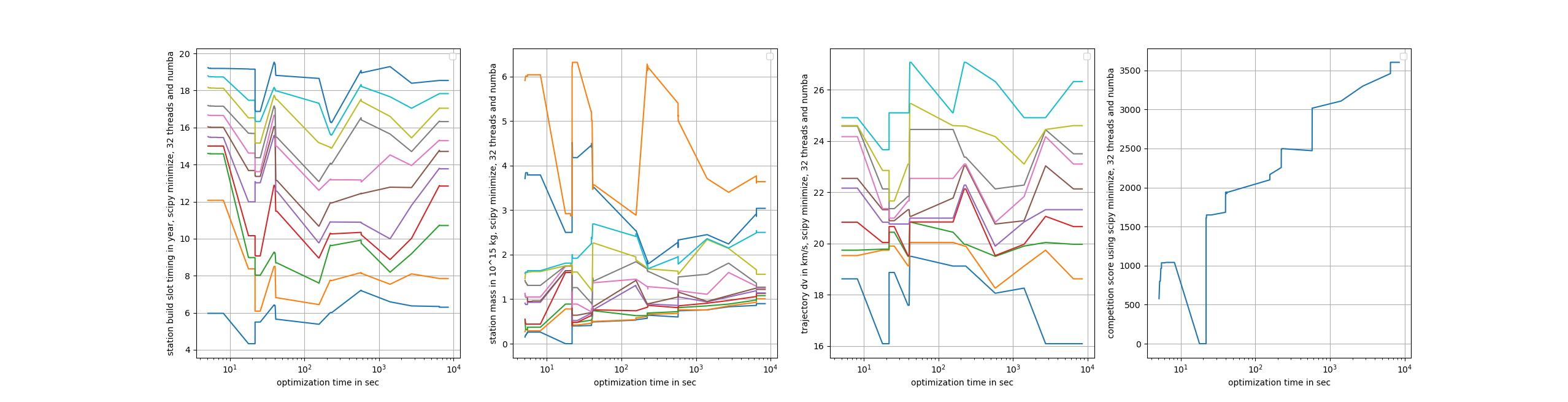
The best scipy algorithm is Dual Annealing.
Writing an objective function in Python with continuous input variables is surprisingly straightforward.
pandas simplifies preprocessing of CSV input data.

1 thread, no NUMA

The following results were obtained with single-threaded optimization after commenting out all @njit annotations to disable Numba. This causes a dramatic loss of performance of roughly 450x.

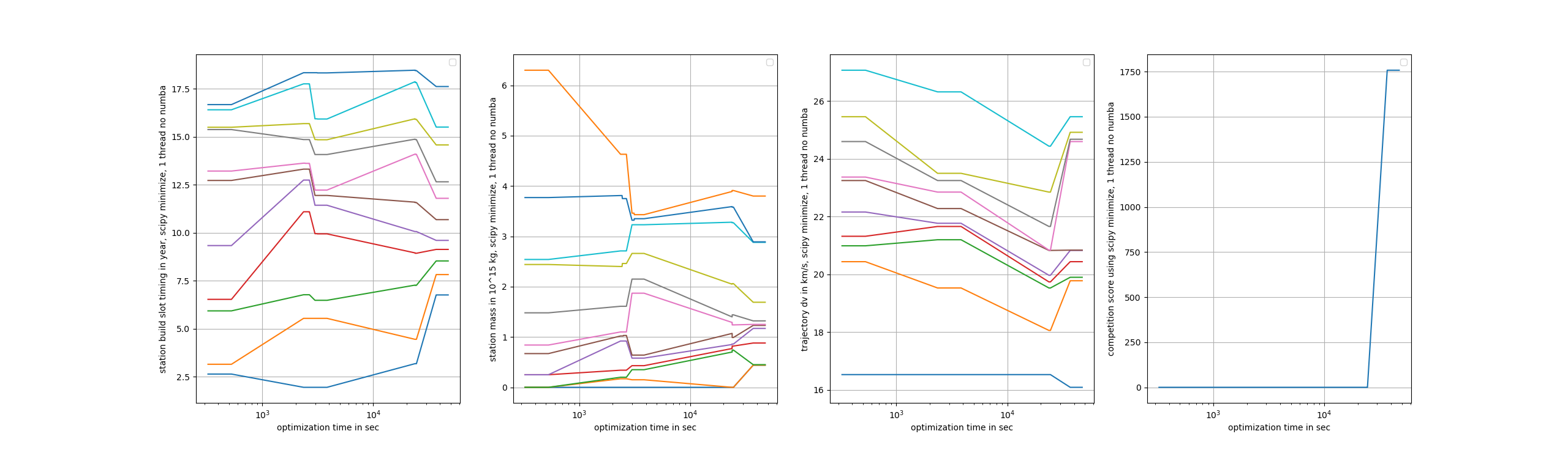
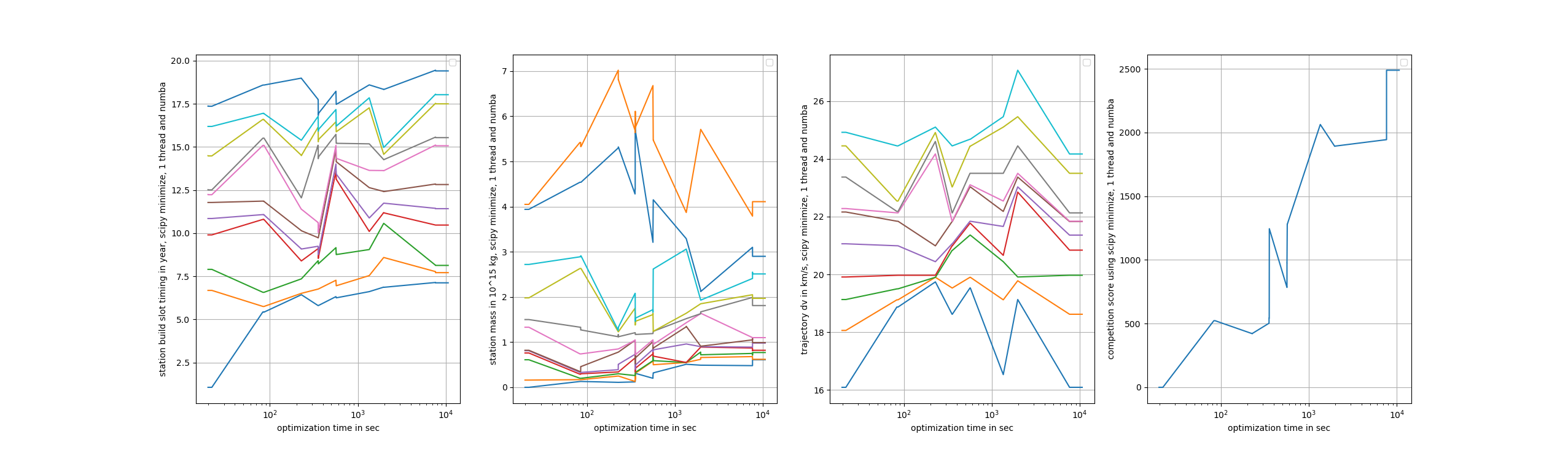
scipy minimize should be avoided for scheduling problems:

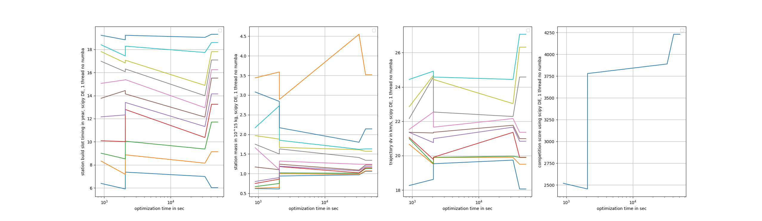
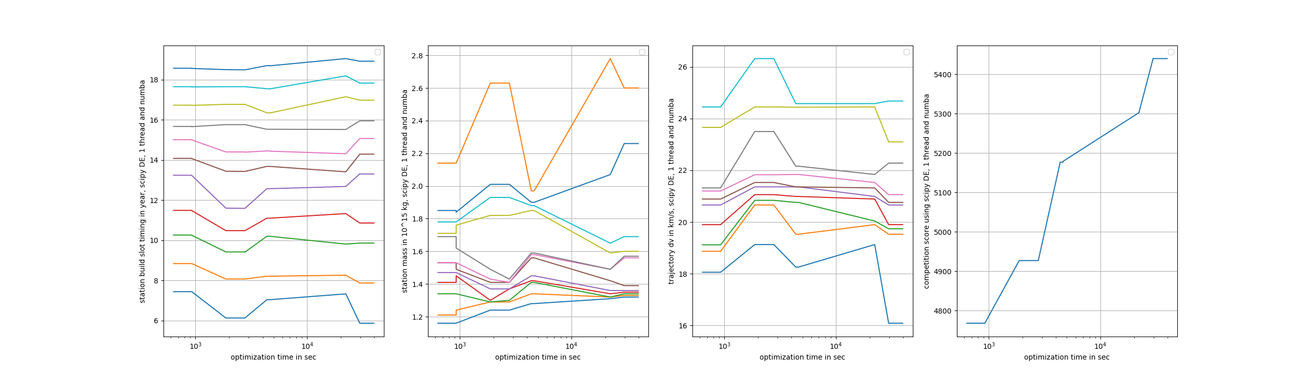
scipy differential_evolution is better, but still not sufficient:

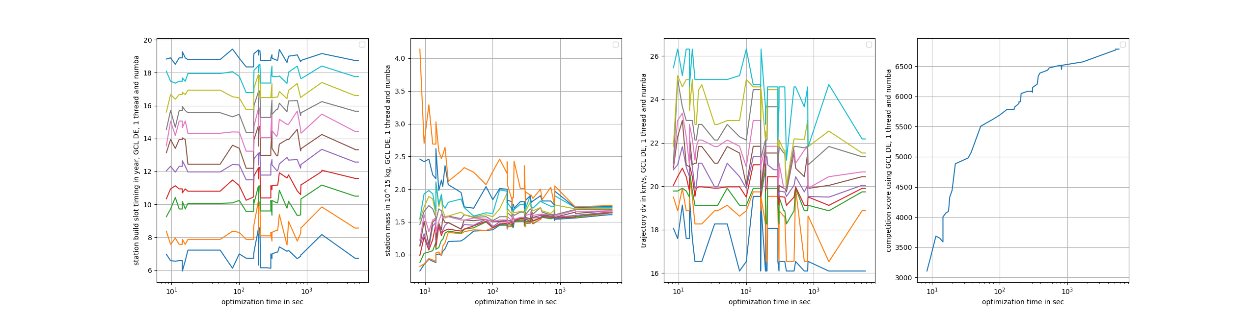
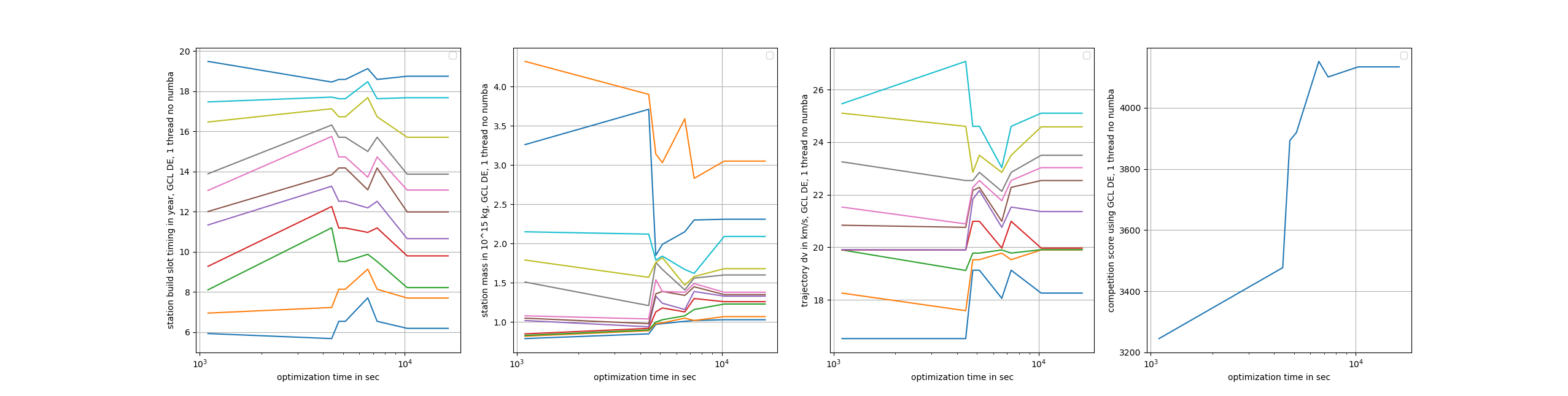
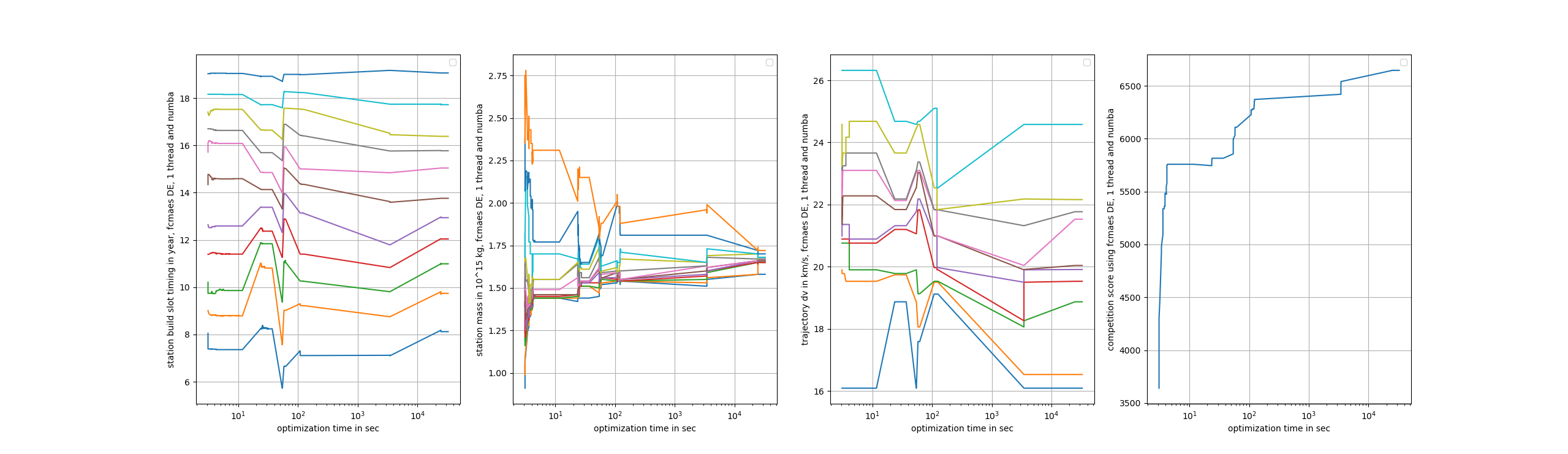
fcmaes GCL DE, another differential evolution variant.

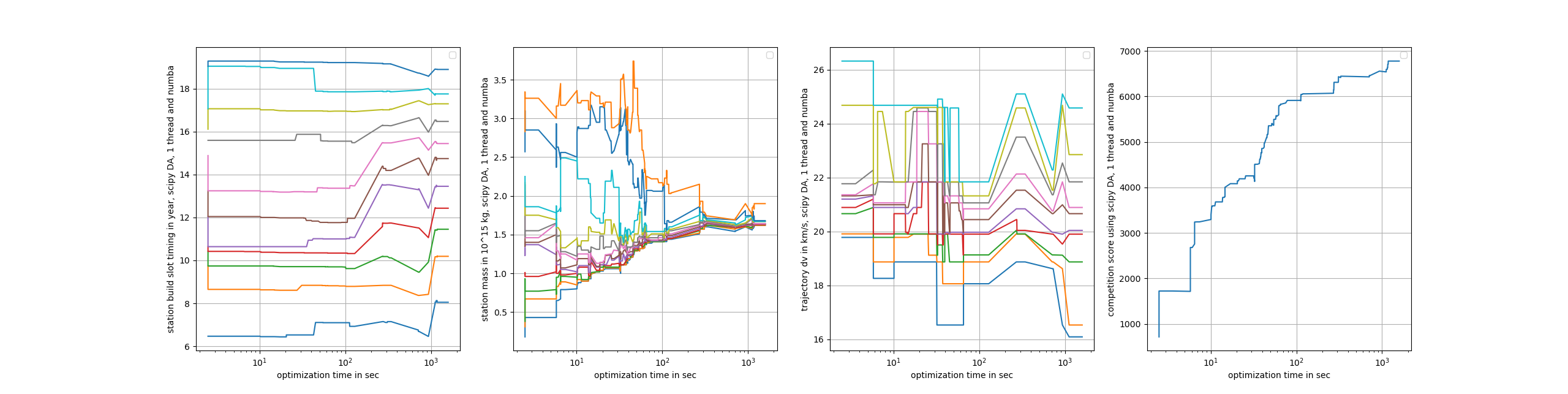
scipy dual_annealing can be used, but is slow:

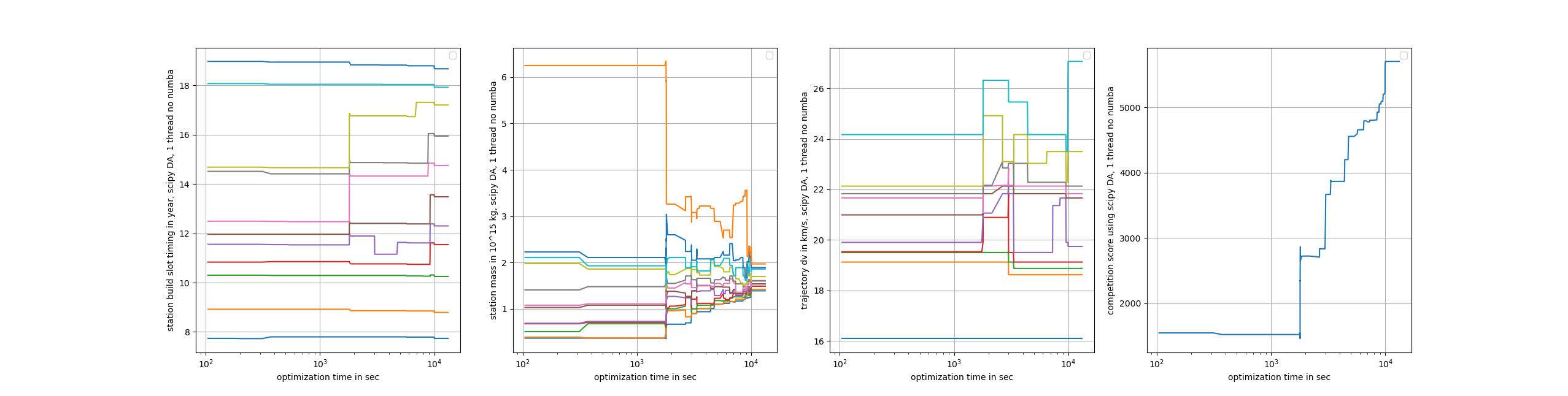
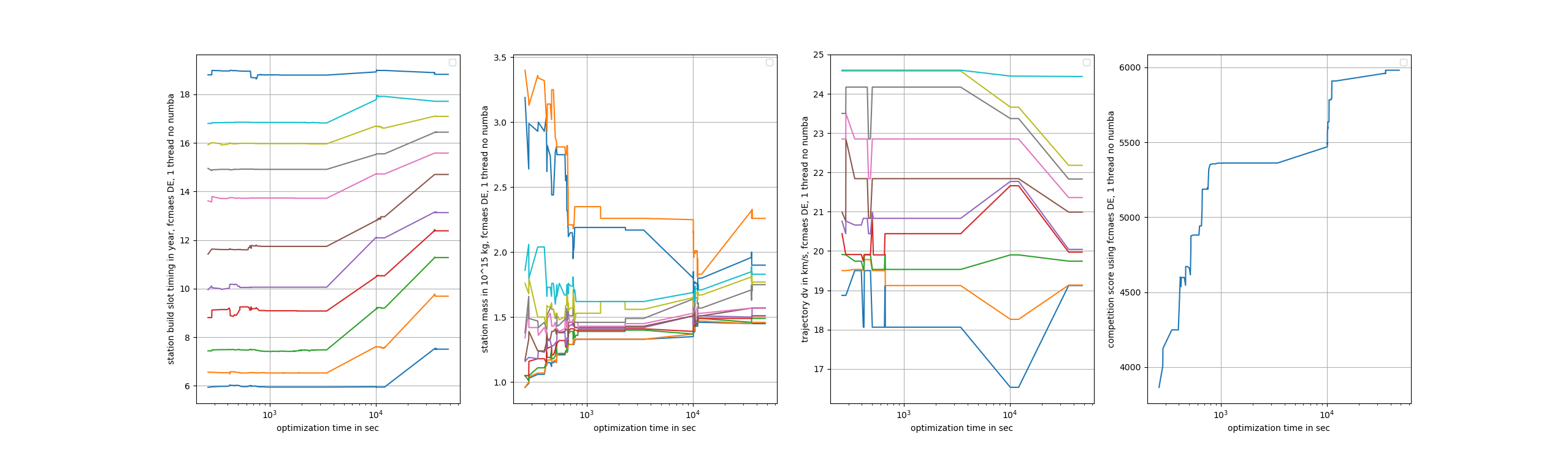
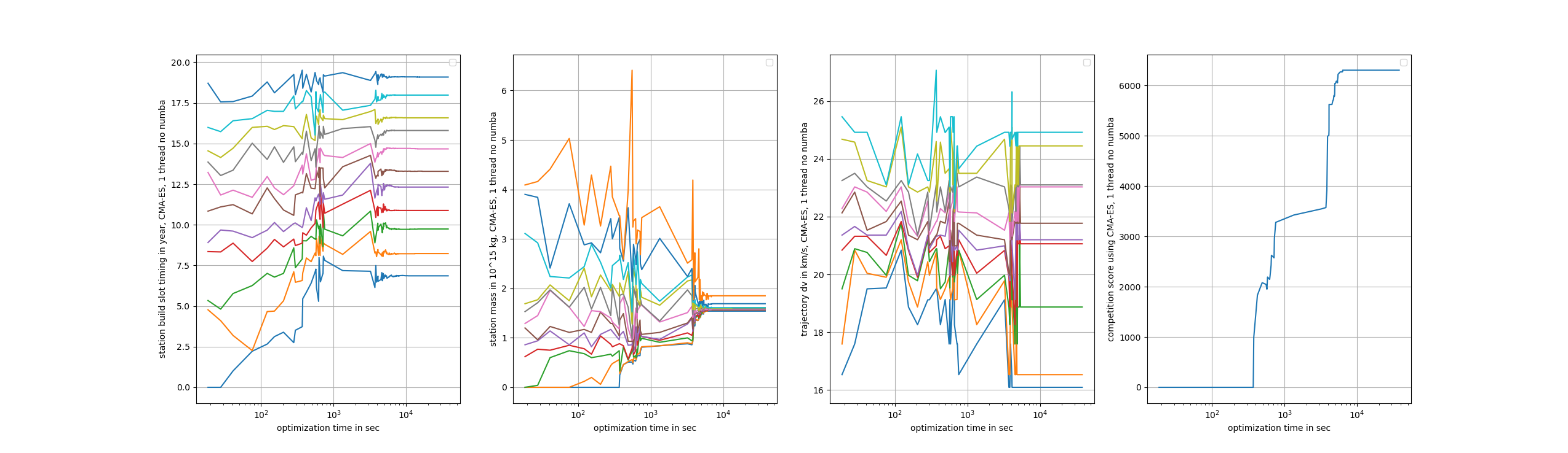
The following algorithms all perform quite well given the small number of function evaluations possible without Numba:

fcmaes differential evolution

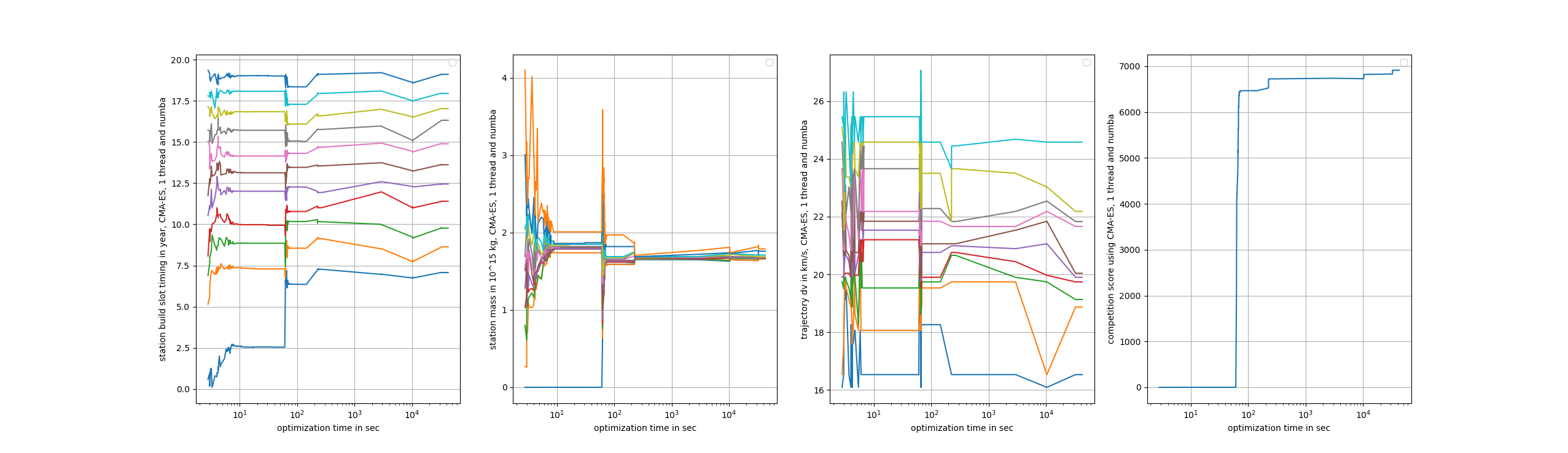
CMA-ES

BiteOpt

1 thread, using NUMA

Once Numba is enabled, results improve significantly. It is still worth noting that algorithms which do not fit the problem well cannot fully exploit the 450x speedup. Even the best of them still need about one hour to find a good solution.

scipy minimize

scipy differential_evolution

scipy dual_annealing

fcmaes differential evolution

fcmaes GCL DE

CMA-ES

BiteOpt

32 threads, using NUMA

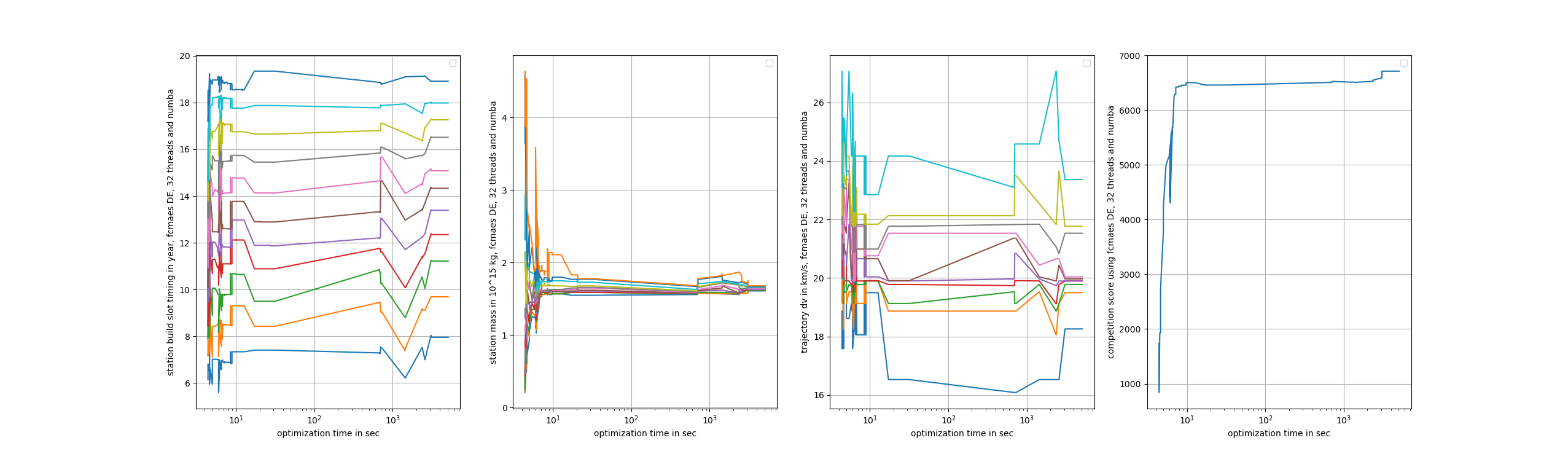
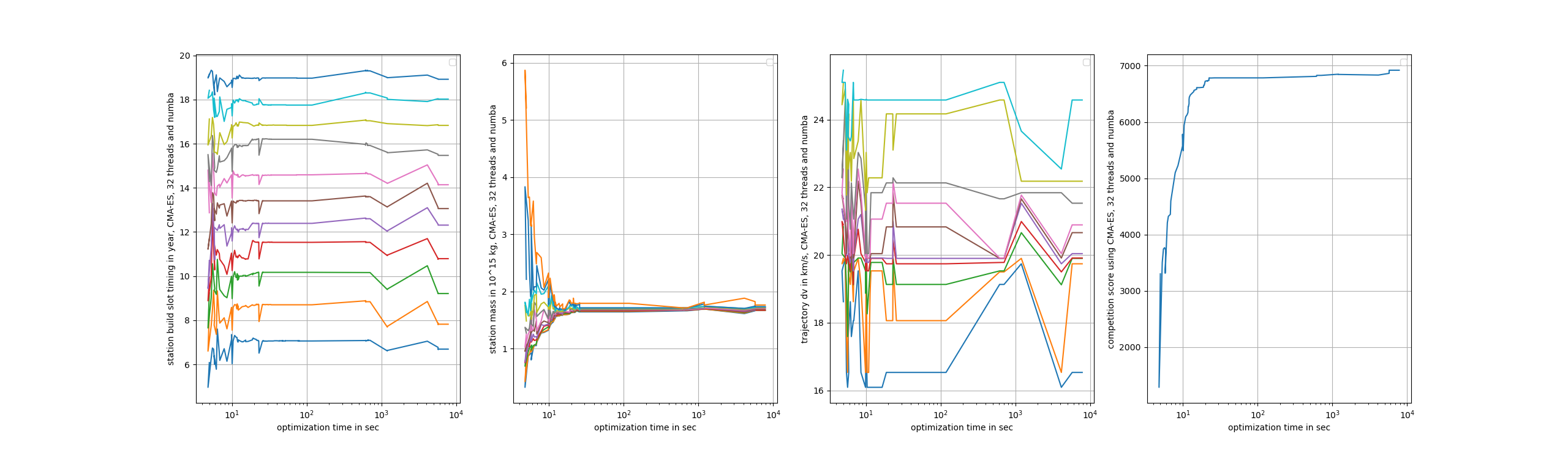
fcmaes provides a parallel retry mechanism that runs many optimization retries in parallel. We used 32 parallel threads on a 16 core AMD 5950x CPU. The speedup from parallelization is between 8x and 18x, depending on the algorithm. At this point, BiteOpt, CMA-ES, and scipy Dual Annealing all produce very good results.

scipy minimize

scipy dual_annealing

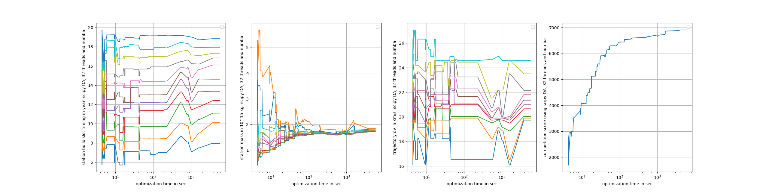
fcmaes differential evolution

CMA-ES

BiteOpt

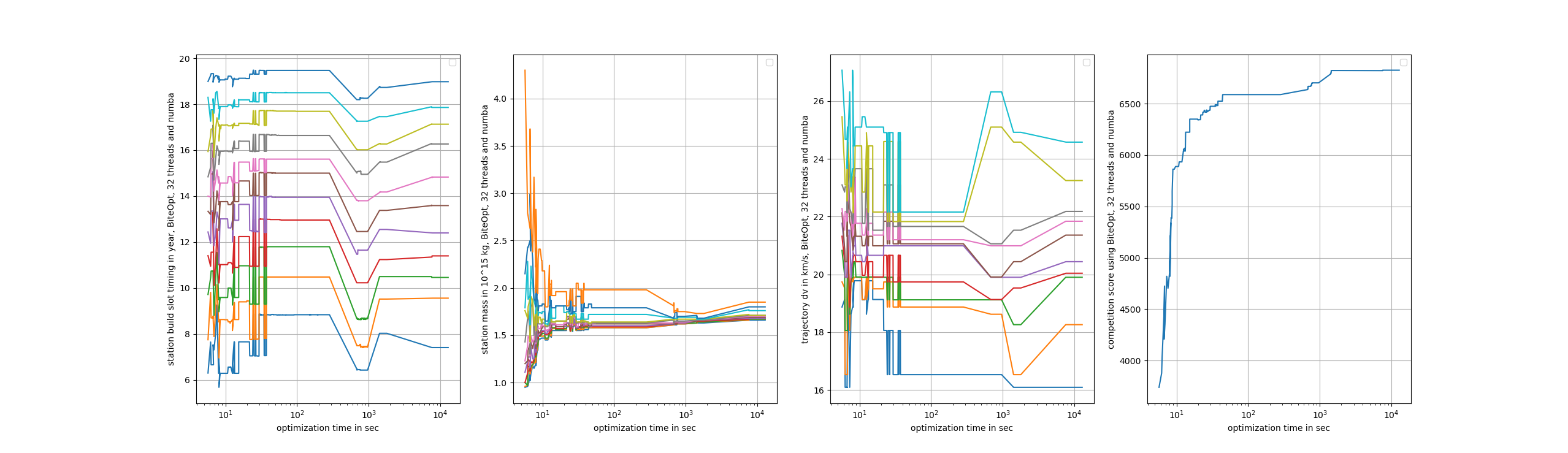
32 threads, Smart Boundary Management using NUMA

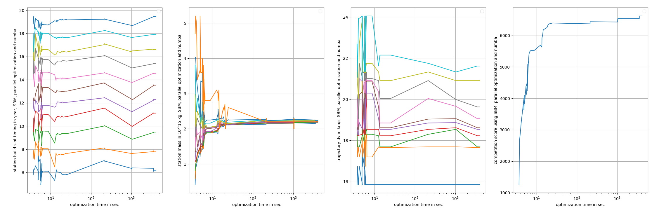
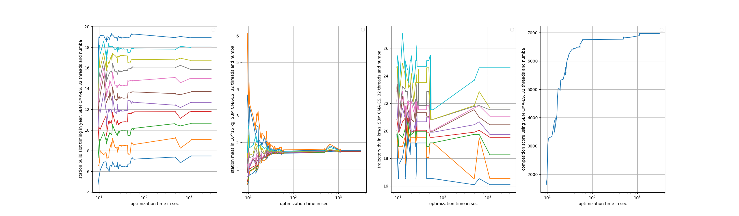
One algorithm that fits this problem especially well is the fcmaes smart boundary management parallel meta-algorithm. We applied it to its default base algorithm, a DE→CMA-ES sequence, as well as to BiteOpt and to CMA-ES alone. BiteOpt is not a particularly good match here. The other two base algorithms perform better. Only a few seconds are needed to obtain a good result, and the optimum is found after about 1 hour.

fcmaes SBM applied to DE→CMA-ES

fcmaes SBM applied to BiteOpt

fcmaes SBM applied to CMA-ES

16 threads, Multi-objective optimization (modecpp) using NUMA

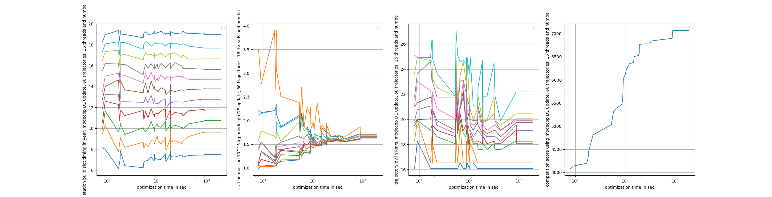
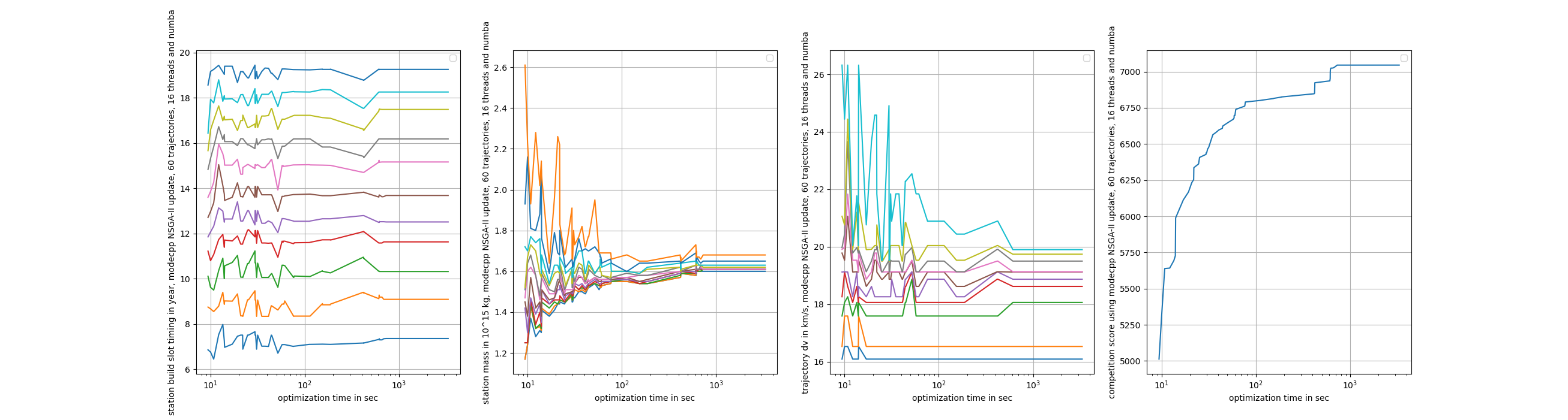
Somewhat surprisingly, the algorithm that fits this problem best is the fcmaes modecpp multi-objective optimizer applied to the single-objective "score". The real objective is hidden from modecpp, but optimizing the two objectives "maximal mass" and "minimal dv value" guides the search effectively.

modecpp parallel retry using DE population update (score 7067):

modecpp parallel retry using NSGA-II population update (score 7045):

modecpp parallel retry using DE population update, 120 trajectories (score 7203):

What about the competition ?

There are not many open source optimization libraries that match fcmaes in their support for parallelization, multiple objectives, constraints, and mixed-integer problems. pymoo meets these requirements, has excellent documentation, and is easy to use. The only slightly tricky point here is that numba does not support mixed integer arrays. We therefore use x.astype(float) to convert the decision variables to a float array.

def check_pymoo(dim, fit, lb, ub, is_MO):
    ...
    if is_MO:
        lb[:10] = 0
        ub[:10] = TRAJECTORY_NUM-1 # integer variables include upper bound

    class MyProblem(ElementwiseProblem):

        def __init__(self, **kwargs):
            super().__init__(n_var=dim,
                             n_obj=2,
                             n_constr=0,
                             xl=np.array(lb),
                             xu=np.array(ub), **kwargs)

        def _evaluate(self, x, out, *args, **kwargs):
            if is_MO:
                out["F"] = fit.fun(x.astype(float)) # numba requires all floats
            else:
                out["F"] = fit(x.astype(float))  #  fit returns the score

    pool = ThreadPool(16)
    problem = MyProblem(runner=pool.starmap, func_eval=starmap_parallelized_eval)

    mask = ["int"]*10+["real"]*(dim-10)

    sampling = MixedVariableSampling(mask, {
        "real": get_sampling("real_random"),
        "int": get_sampling("int_random")
    })

    crossover = MixedVariableCrossover(mask, {
        "real": get_crossover("real_sbx", prob=0.9, eta=15),
        "int": get_crossover("int_sbx", prob=0.9, eta=15)
    })

    mutation = MixedVariableMutation(mask, {
        "real": get_mutation("real_pm", eta=20),
        "int": get_mutation("int_pm", eta=20)
    })

    if is_MO:
        algorithm = NSGA2(
            pop_size=256,
            n_offsprings=10,
            sampling=sampling,
            crossover=crossover,
            mutation=mutation,
            eliminate_duplicates=True
        )
    else:
        algorithm = DE(
            pop_size=100,
            variant="DE/rand/1/bin",
            CR=0.3,
            dither="vector",
        )

    from pymoo.optimize import minimize

    res = minimize(problem,
                   algorithm,
                   get_termination("n_gen", 500000),
                   verbose=False)

You can get reasonable results quickly, but I never found a score > 7000 using pymoo. The number of evaluations per second is much lower than with fcmaes, partly because pymoo can parallelize only function evaluations, not complete optimization runs. As with fcmaes, the multi-objective results from NSGA2 are better than the results from single-objective optimization with DE. Unfortunately, specifying MixedVariableSampling for DE leads to an error. So does pool = multiprocessing.Pool(16).

Conclusion

There are four main conclusions:

Do not be afraid to add decision variables to your objective function. Almost all GTOC11 participants chose the opposite approach and solved the problem incrementally, step by step. That limits what the optimizer can do. More decision variables make the problem harder, but they also create new opportunities. Do not underestimate what the optimizer can achieve.
If your final target is a single objective, such as the GTOC11 score, but that score is derived from several objectives, also try a multi-objective optimizer. It may produce a more diverse set of solutions and, as shown here, it may even improve the final single-objective score. This result was confirmed with both fcmaes and pymoo.
Python is suitable for expensive objective functions, but only if you use numba where it fits. Pure NumPy matrix operations can work without it. As soon as loops are involved, numba is necessary if you want to stay competitive with C++.
Try to use all CPU cores and threads available. GTOC11 participants often used GPUs because of their very high core counts. That makes sense for building the database or table used as the basis of the optimization. For the optimization itself we are currently limited to CPU cores. There are two options: parallel objective-function evaluation and parallel optimization runs. The second option usually scales better and was advantageous for GTOC11.

The suitability of an optimization algorithm for a competition such as GTOC11, which is a real-world application, cannot be judged from standard single-threaded benchmarks that ignore parallelism. Standard benchmarks are useful for finding errors, but not for tuning your algorithms. For example, standard pymoo algorithms such as DE or NSGA2 find reasonable solutions quickly, but they do not scale well with the time or evaluation budget, and they do not scale well with the number of available CPU cores.