

One To Rule Them All
This tutorial
-
Applies a new combination of optimization algorithms, CR-FM-NES and BiteOpt, in sequence to different scheduling and packing problems of practical relevance: MMKP and VRPTW.
-
Compares the results for typical benchmark problems to reference solutions.
-
Shows how to define efficient fitness functions for these problems in Python.
-
Discusses when to apply the new method.
Motivation
While experimenting with problems that use discrete decision variables, such as scheduling and packing, two optimization algorithms stood out: CR-FM-NES and BiteOpt.
-
Minimal algorithmic overhead, even with a large number of decision variables (> 1000).
-
High diversity across multiple runs.
-
Good resilience on discontinuous, multi-modal, or noisy objective functions.
-
Good support for integer decision variables. We convert continuous variables using numpy’s
argsortorastype(int).
CR-FM-NES converges faster. BiteOpt is better at escaping local minima. In a parallel retry setting, it is therefore natural to run CR-FM-NES first and then use its result as the initial guess for BiteOpt.
We tried this CR-FM-NES → BiteOpt sequence for Multi-UAV Task Assignment. There it outperformed several problem-specific algorithm implementations such as GA, PSO, and ACO.
In this tutorial, we extend that idea to MMKP and VRPTW, two very different problems with high practical relevance.
Do we need a problem specific optimization algorithm
Traditionally, even when heuristic methods are used, the optimizer is designed for one specific problem. See UAV1, for example, where three heuristic approaches, GA, ACO, and PSO, are compared. We already showed in a fork, UAV2, that results may improve when we give up this idea and apply a generic algorithm instead.
Packing, scheduling, and vehicle routing all have many practically relevant variants. Adapting and reimplementing successful algorithms for each new variant is demanding. In vehicle routing, more generic approaches already exist that cover multiple variants: A generic exact solver for vehicle routing and related problems. Better still would be to avoid creating a problem-specific algorithm entirely.
In that case, we only need an efficient implementation of the objective function, the "scoring" of a solution. That part can often be adapted more easily to many variants. Such a "one for all" approach is useful in several situations:
-
We face a very specific problem variant and do not have a good algorithm for it.
-
Our programming skills are sufficient to code an objective function in Python, but not to build a problem-specific solver.
-
We want to avoid learning the complex API of a problem-specific solver such as or-tools or OptaPlanner.
-
There is no good open source solution for our specific problem in the programming language we want to use.
-
We have multiple competing objectives and want the pareto front of non-dominated choices.
To study the tradeoff, "how much do we lose with the generic approach", we can test it on well-known problem variants where researchers had decades to improve specialized algorithms. MMKP and VRPTW are good candidates because they are important in practice and heavily studied. Still, we do not see these benchmark problems as the main application area of the approach.
Optimization needs to be "tweaked" to support parallelism
CPU vendors are investing in many-core architectures, and cloud computing offers affordable large-scale parallelism. This trend extends the reach of continuous optimization far beyond its traditional application areas. In this setting, optimization algorithms need different tuning. High diversity across repeated runs becomes much more important. This may explain why the CR-FM-NES → BiteOpt sequence performs better than the alternatives we tried.
Note: CR-FM-NES does not have this property in general. We need to lower the initial step size parameter input_sigma.
Note: The fcmaes implementation of parallelism works much better on Linux. On Windows, consider using the Linux subsystem for Windows WSL.
MMKP Multiple-choice Multidimensional Knapsack Problem
MMKP is a knapsack and packing problem of practical importance because several real-world optimization problems can be mapped to it. Examples are:
-
Quality of service management for timeliness, reliability, security, and related criteria.
-
Optimal number of warehouses needed to store a set of items while preventing incompatible items from being stored together.
Problem description
We have n sets composed of mutually exclusive items. The goal is to select exactly one item from each set and maximize the overall value without violating a family of resource constraints. For each resource, the sum of the resource values of the chosen items must not exceed a resource-specific threshold.
See MMKP-Ants for the mathematical details.
Note: Hard multidimensional multiple choice knapsack problems states: "An instance is hard to solve when all classes contain the same profit vector and the weights are correlated with the profits". The selection of benchmark problems may influence the results.
Reference solutions
We use the well-known MMKP benchmark problems "I01-I13", which are cited in most related publications. The literature reports excellent results (see hybrid algorithm), but we did not find the corresponding solution instances. We therefore applied Simulated Annealing for 1E8 iterations with multiple retries to produce at least some kind of "reference solutions", which can be verified:
| problem | score | deviation from optimum |
|---|---|---|
I01 |
173.0 |
0.0 |
I02 |
364.0 |
0.0 |
I03 |
1597.0 |
0.31 |
I04 |
3581.0 |
0.44 |
I05 |
3905.7 |
0.0 |
I06 |
4799.3 |
0.0 |
I07 |
24410.0 |
0.8 |
I08 |
36577.0 |
0.89 |
I09 |
48742.0 |
0.92 |
I10 |
60902.0 |
0.95 |
I11 |
73139.0 |
0.89 |
I12 |
85261.0 |
0.97 |
I13 |
97712.0 |
0.75 |
Note that both hybrid algorithm and Hifi report better solutions. The latter used a 250 Mhz CPU with 128 Mb of RAM and generated an I13 result of 98429 in 160 seconds single-threaded. Please contact me if you know where the corresponding code can be found.
Benchmark results for continuous optimization
These benchmark results for continuous optimization were computed on a 16 core AMD 5950x CPU using 32 parallel threads with the code at mmkp.py:
| problem | score | deviation from optimum | time in seconds | time to reach 2% deviation |
|---|---|---|---|---|
I01 |
173.0 |
0.0 |
0.59 |
0.59 |
I02 |
364.0 |
0.0 |
0.22 |
0.22 |
I03 |
1602.0 |
0.0 |
124 |
20 |
I04 |
3572.0 |
0.7 |
416 |
21 |
I05 |
3905.7 |
0.0 |
0.67 |
0.57 |
I06 |
4799.3 |
0.0 |
0.95 |
0.8 |
I07 |
24232.0 |
1.53 |
451 |
8 |
I08 |
36411.0 |
1.34 |
1800 |
18 |
I09 |
48503.0 |
1.4 |
1859 |
23 |
I10 |
60611.0 |
1.42 |
1727 |
35 |
I11 |
72745.0 |
1.43 |
5713 |
51 |
I12 |
84928.0 |
1.36 |
3983 |
74 |
I13 |
97077.0 |
1.39 |
2342 |
95 |
As you can see, we lose about 0.5% accuracy compared to the reference solutions above. We still reach 2% accuracy in less than a minute, even for the larger instances. The following diagram shows the relation between the number of groups or decision variables and the time to reach 2% accuracy:
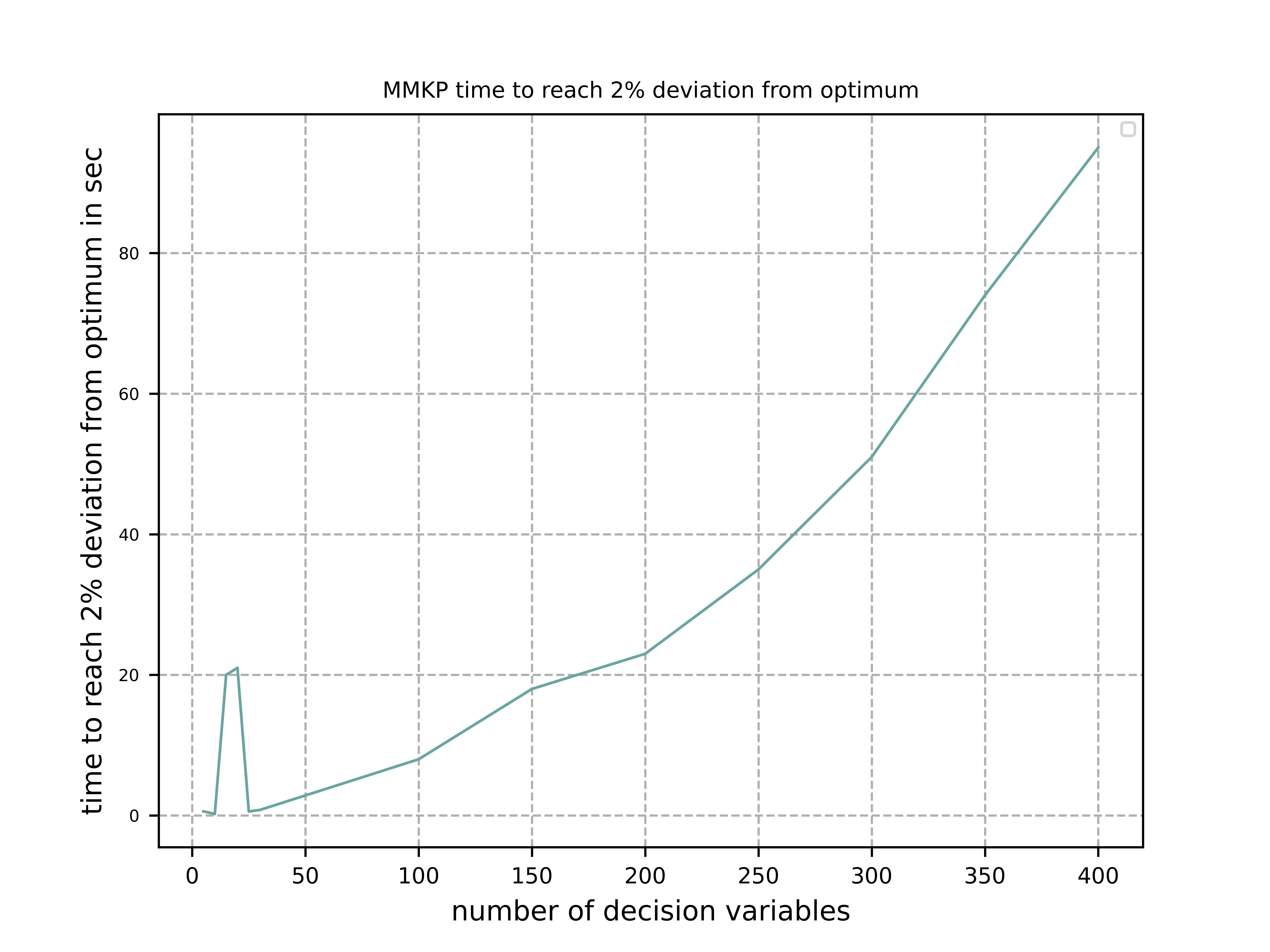
The relation is almost linear. That suggests we can handle even larger instances with reasonable effort.
Alternative approaches
Github repositories related to MMKP are:
-
Simulated Annealing C++ algorithm solving the problem slightly better than our approach. But it is MMKP-specific, and you need to implement some interface if you want to use it from Python.
-
MMKP Heuristics. A nice comparison of different older C++ algorithms, none of which seems to work better than Simulated Annealing.
Both hybrid algorithm and Hifi report better results, but there seems to be no related open source code available.
Implementation
The complete code for the MMKP problem is at mmkp.py.
To apply continuous optimization, we represent a problem instance as Python class MMKP:
class MMKP():
    def __init__(self, problem):
        self.problem = problem
        filename = 'problems/' + problem
        self.n, self.l, self.m, self.best_val, self.best_sol,\
                self.avail, self.values, self.resources = parse(filename)
        self.dim = self.n
        self.bounds = Bounds([0]*self.dim, [self.l-1E-12]*self.dim)

    def fitness(self, x):
        vsum, penalty = fitness_(x.astype(int), self.n, self.l, self.avail, \
                self.values, self.resources)
        if penalty > 0:
            penalty += 100
        return self.deviation(vsum) + penalty
We extract the problem parameters by parsing the instance file:
-
Available resources:
self.avail -
Resource consumption for each item:
self.resources -
Value of each item:
self.values -
Reference solution value:
self.best_val -
Number of groups:
self.n -
Number of items to choose from per group:
self.l
The number of decision variables, self.dim, is equal to the number of groups. The boundaries are [0, self.l-1E-12]. The fitness function maps each continuous decision vector to a vector of integers in the [0, self.l-1] interval using numpy’s astype(int). These integers represent the selected item for each group. fitness delegates to a fast numba function, fitness_, which checks resource consumption and returns the overall value together with a penalty value for resource violations.
@njit(fastmath=True)
def fitness_(x, n, l, avail, values, resources):
    vsum = 0
    rsum = np.zeros(l, dtype=numba.int32)
    for i in range(n):
        vsum += values[i][x[i]]
        rsum += resources[i][x[i]]
    rsum = np.maximum(rsum - avail, np.zeros(l, dtype=numba.int32))
    pen = np.sum(rsum)
    return vsum, pen
Problem variants
This function is much easier to adapt to problem variants than optimization algorithms that use the "internal structure" of a problem instance. Those algorithms usually support incremental changes of a solution by computing the score delta. See for instance saMultiChoiceKnapsack.cpp.
As an example, assume we want not only to maximize the sum of item values, but also to achieve balanced resource consumption. We can express this by the standard deviation of the consumed resources divided by their availability. Only a small modification of the fitness or objective function is required:
@njit(fastmath=True)
def fitness_(x, n, l, avail, values, resources):
    vsum = 0
    rsum = np.zeros(l, dtype=numba.int32)
    for i in range(n):
        vsum += values[i][x[i]]
        rsum += resources[i][x[i]]
    sdev = np.std(rsum/avail)
    rsum = np.maximum(rsum - avail, np.zeros(l, dtype=numba.int32))
    pen = np.sum(rsum)
    return vsum, pen, sdev

...
    def fitness(self, x):
        vsum, penalty, sdev = fitness_(x.astype(int), self.n, self.l, self.avail, \
                self.values, self.resources)
        if penalty > 0:
            penalty += 100
        return self.deviation(vsum) + penalty + 10*sdev
We applied a specific weight 10 to the standard deviation. For smaller problem instances, we could instead apply a multi-objective algorithm to generate the complete pareto front. That algorithm also comes with fcmaes and is used in many other tutorials.
Exercise
Apply the same modification to saMultiChoiceKnapsack.cpp. Hint: This may be a bit tricky. Note that this optimization algorithm is not only problem-specific, it is benchmark-specific.
It exploits the fact that for most benchmarks the resource limit for all resources is equal.
Here
double ratio = value/weight the resource consumption weight
is not normalized using the resource availability as it should be.
MMKP Optimization
Parallelization of optimization runs and of the optimization algorithm comes for free if we use the fcmaes library:
stop_fitness = 2.0
popsize = 500

opt = crfmnes_bite(max_evaluations, popsize=popsize, M=4, stop_fitness = stop_fitness)

def optimize(mmkp, opt, num_retries = 32):
    ret = retry.minimize(wrapper(mmkp.fitness),
                               mmkp.bounds, num_retries = num_retries,
stop_fitness = stop_fitness, optimizer=opt)-
crfmnes_biterepresents a sequence of CR-FM-NES and BiteOpt. -
wrappermonitors and logs the progress for all parallel runs. -
stop_fitnesstells the algorithm to stop when a specific value or deviation is reached. -
popsizeandMare configuration parameters of the used optimizers.
These settings are sufficient if you aim for a 2% deviation from the optimum (stop_fitness = 2.0). A 1.5% deviation is much harder to achieve, so you may want to increase the number of retries, num_retries. The number of parallel retries depends on the CPU. For the AMD 5950x it is 32, and this can be overwritten using the workers argument. We experimented with smaller population sizes for smaller instances, but there is not much to gain. Both CR-FM-NES and BiteOpt are largely self-adapting.
VRPTW capacitated Vehicle Routing Problem with Time Windows
VRPTW is a variant of the vehicle routing problem for multiple vehicles with customer demands, capacity constraints, time windows, and customer service times. Because of its practical relevance, it is one of the best-studied optimization problems in computer science. There is a large body of literature, many sophisticated problem-specific algorithms, and benchmark sets with reference solutions proven to be optimal. See https://developers.google.com/optimization/routing/vrp for a nice introduction.
Open source libraries such as or-tools provide a vehicle-routing-specific API and produce nearly perfect results (see VRPTW results).
The "optimization without a problem-specific optimizer" approach should not be applied here if the standard problem is all you need. Still, it is interesting to measure how much we lose when we try it anyway. The code can also be adapted easily to other variants with additional constraints or different objectives. That is where this approach is most useful.
Problem description
We plan routes for a fleet of vehicles to serve a set of customer demands. Each vehicle has a capacity constraint on the total demand it serves. Each customer node has a time window, and customer-specific service times must be considered. Possible objectives are the number of vehicles used and the overall distance traveled by all vehicles. If only one vehicle is available, the problem becomes a variant of TSP, the Traveling Salesman Problem.
Possible variants include variable vehicle speed, noisy distances or demands, and additional constraints.
Benchmarks
Many different benchmarks are used in the literature. We choose the 100-customer instances of Solomon’s benchmark http://web.cba.neu.edu/~msolomon/problems.htm because reference solutions are available and the benchmark is cited in most related publications.
There are two different objectives for Solomon’s VRPTW benchmark:
The single-objective variant can be solved almost perfectly using or-tools, so we choose that one. See optimize_or.py for the or-tools implementation used to generate the reference results for comparison here. We found other reference solutions at galgos, but some of them did not pass our validation. These solutions assume rounding of the distances, which makes them incompatible with the interpretation of the problem used here.
Alternative implementations
Besides optimize_or.py, there are many implementations for this problem. http://vrp.galgos.inf.puc-rio.br/index.php/en/links links to some of them. That is not the case for optimization without a problem-specific algorithm. Maybe that is because most continuous optimization algorithms do not work well here.
Implementation
The complete code for the VRPTW problem is at vrptw.py. To apply continuous optimization, we represent a problem instance as Python class VRPTW:
class VRPTW():
    def __init__(self, problem):
        self.problem = problem
        filename = 'problems/' + problem + '.txt'
        self.vnumber, self.capacity, self.dtime, self.demand, self.ready,\
            self.due, self.service = parse_problem(filename)
        self.dim = len(self.demand) - 1
        self.bounds = Bounds([0]*self.dim, [1]*self.dim)

    def fitness(self, x):
        fit = fitness_(np.argsort(x), self.capacity, self.dtime, self.demand, \
                    self.ready, self.due, self.service)
        return 10*fit[0] + fit[1]
We extract the problem parameters by parsing the instance file:
-
Vehicle capacities:
self.capacity -
Distance matrix:
self.dtime -
Customer demand:
self.demand -
Customer is ready time:
self.ready -
Customer due time:
self.due -
Customer service time:
self.service
The number of decision variables, self.dim, is equal to the number of customer locations.
Note that all tables include a 0-entry for the start and end location.
We use the [0, 1] interval as boundary. The fitness function converts the continuous argument vector into a list of unique integers using np.argsort(x).
fitness then delegates to a fast numba function, fitness_, which executes all tours and evaluates both the objectives and the constraints.
Instead of ignoring the vehicle number, we include it with some weight, even though we are ultimately interested only in the overall distance. This acts as a heuristic that supports the optimization process. We observed that good solutions usually use a fairly low number of vehicles.
@njit(fastmath=True)
def fitness_(seq, capacity, dtime, demands, readys, dues, services):
    n = len(seq)
    seq += 1
    sum_demand = 0
    sum_dtime = 0
    time = 0
    last = 0
    vehicles = 1
    for i in range(0, n+1):
        customer = seq[i] if i < n else 0
        demand = demands[customer]
        ready = readys[customer]
        due = dues[customer]
        service = services[customer]
        if sum_demand + demand > capacity or \
                time + dtime[last, customer] > due:
            # end vehicle tour, return to base
            dt = dtime[last, 0]
            sum_dtime += dt
            time = 0
            sum_demand = 0
            vehicles += 1
            last = 0
        # go to customer
        dt = dtime[last, customer]
        time += dt
        if time < ready:
            time = ready
        time += service
        sum_demand += demand
        sum_dtime += dt
        last = customer
    return np.array([float(vehicles), sum_dtime])
VRPTW Optimization
You will probably notice that this code is almost exactly the same as for MMKP above.
Even the popsize parameter is the same.
popsize = 500
opt = crfmnes_bite(max_evaluations, popsize=popsize, M=4)

def optimize(vrptw, opt, num_retries = 64):
    ret = retry.minimize(wrapper(vrptw.fitness),
vrptw.bounds, num_retries = num_retries, optimizer=opt)-
crfmnes_biterepresents a sequence of CR-FM-NES and BiteOpt. -
wrappermonitors and logs the progress for all parallel runs. -
popsizeandMare configuration parameters of the used optimizers.
Exercise
Modify the fitness function to handle a problem variant with noisy demands.
For example, when using demands[customer], multiply it with a random factor in the [0.8,1.2] interval.
You then need to call fitness_ multiple times and use a "worst case" value as the fitness.
See link:TSP.html where this was done for TSP.
Can you do the same using or-tools by modifying
optimize_or.py?
Results
Continuous optimization is performed by a sequence of CR-FM-NES and BiteOpt, with 64 runs in total and 32 runs performed in parallel. On an AMD 5950x 16 core CPU, this takes about 7 minutes.
Compared to the or-tools result, which serves as the reference, we lose about 0.2% on the clustered problem instances and about 3% on the random problem instances.
| optimizer | C1 | C2 | R1 | R2 | RC1 | RC2 |
|---|---|---|---|---|---|---|
or-tools |
828.4 |
589.9 |
1182.6 |
878.0 |
1360.9 |
1005.3 |
continuous |
829.3 |
591.8 |
1221.6 |
909.7 |
1384.2 |
1035.2 |
%difference |
0.11 |
0.34 |
3.3 |
3.61 |
1.71 |
2.97 |
| optimizer | C1 | C2 | R1 | R2 | RC1 | RC2 |
|---|---|---|---|---|---|---|
or-tools |
10.0 |
3.0 |
13.33 |
5.45 |
13.12 |
6.25 |
continuous |
10.0 |
3.0 |
14.0 |
5.36 |
13.88 |
6.75 |
%difference |
0.0 |
0.0 |
5.0 |
-1.67 |
5.71 |
8.0 |
| problem | vehicles | distance | % vehicles difference | % distance difference |
|---|---|---|---|---|
c101 |
10 |
828.9 |
0.0 |
-0.0 |
c102 |
10 |
828.9 |
0.0 |
0.0 |
c103 |
10 |
830.2 |
0.0 |
0.26 |
c104 |
10 |
831.1 |
0.0 |
0.77 |
c105 |
10 |
828.9 |
0.0 |
-0.0 |
c106 |
10 |
828.9 |
0.0 |
-0.0 |
c107 |
10 |
828.9 |
0.0 |
-0.0 |
c108 |
10 |
828.9 |
0.0 |
-0.0 |
c109 |
10 |
828.9 |
0.0 |
-0.0 |
c201 |
3 |
591.6 |
0.0 |
-0.0 |
c202 |
3 |
591.6 |
0.0 |
0.0 |
c203 |
3 |
594.7 |
0.0 |
0.6 |
c204 |
3 |
603.0 |
0.0 |
2.09 |
c205 |
3 |
588.9 |
0.0 |
-0.0 |
c206 |
3 |
588.5 |
0.0 |
-0.0 |
c207 |
3 |
588.3 |
0.0 |
0.0 |
c208 |
3 |
588.3 |
0.0 |
0.0 |
r101 |
20 |
1670.4 |
0.0 |
1.64 |
r102 |
18 |
1501.8 |
0.0 |
1.97 |
r103 |
15 |
1246.5 |
7.14 |
2.71 |
r104 |
12 |
1024.1 |
9.09 |
4.1 |
r105 |
16 |
1407.9 |
6.67 |
3.46 |
r106 |
14 |
1289.2 |
7.69 |
3.91 |
r107 |
12 |
1119.3 |
9.09 |
3.88 |
r108 |
11 |
990.1 |
0.0 |
3.87 |
r109 |
14 |
1202.8 |
7.69 |
4.42 |
r110 |
13 |
1116.0 |
8.33 |
3.0 |
r111 |
12 |
1083.0 |
0.0 |
2.69 |
r112 |
11 |
1008.6 |
10.0 |
5.53 |
r201 |
8 |
1188.0 |
0.0 |
3.49 |
r202 |
6 |
1067.7 |
-25.0 |
3.01 |
r203 |
6 |
908.7 |
0.0 |
3.78 |
r204 |
5 |
766.7 |
0.0 |
4.2 |
r205 |
5 |
978.8 |
0.0 |
2.38 |
r206 |
4 |
918.8 |
-20.0 |
4.23 |
r207 |
4 |
835.5 |
0.0 |
4.69 |
r208 |
4 |
741.4 |
0.0 |
4.99 |
r209 |
6 |
883.8 |
20.0 |
2.78 |
r210 |
7 |
934.6 |
16.67 |
3.29 |
r211 |
4 |
783.1 |
0.0 |
3.59 |
rc101 |
17 |
1673.5 |
0.0 |
1.59 |
rc102 |
15 |
1490.4 |
7.14 |
0.8 |
rc103 |
13 |
1312.2 |
8.33 |
-0.54 |
rc104 |
11 |
1190.5 |
10.0 |
3.45 |
rc105 |
17 |
1576.5 |
6.25 |
2.9 |
rc106 |
13 |
1401.8 |
0.0 |
1.15 |
rc107 |
13 |
1258.1 |
8.33 |
1.77 |
rc108 |
12 |
1170.6 |
9.09 |
2.96 |
rc201 |
9 |
1297.6 |
0.0 |
2.51 |
rc202 |
8 |
1124.3 |
0.0 |
2.54 |
rc203 |
6 |
974.5 |
20.0 |
4.2 |
rc204 |
5 |
828.5 |
25.0 |
5.35 |
rc205 |
7 |
1176.2 |
0.0 |
1.6 |
rc206 |
7 |
1092.5 |
0.0 |
3.59 |
rc207 |
7 |
982.9 |
16.67 |
1.71 |
rc208 |
5 |
805.4 |
25.0 |
3.25 |
Conclusion
From these results we can conclude:
-
Standard tools like or-tools are hard to beat on the problems they were designed for.
-
For variants with additional constraints, objectives, or noisiness, we first need to check whether those standard tools still apply.
-
Think twice before developing a problem-specific algorithm. It may not be worth the effort if you are not aiming for a perfect solution.
-
The penalty for using a generic optimization method that only requires a fast fitness implementation may be lower than expected, especially when parallelism and recent advances in continuous optimization are taken into account.
-
The CR-FM-NES and BiteOpt sequence proved to be an excellent choice for both vehicle routing (VRPTW) and packing (MMKP) if you want to use Python and take advantage of a modern many-core CPU or multi-node cloud computing resources.