fcmaes - a Python 3 gradient-free optimization library

Simulation Parameter Optimization

Introduction

This tutorial covers one of the most common uses of fcmaes. Suppose you have a simulation that takes several minutes per run. How do you still find good parameter settings?

We use a real example from aging research. The simulation computes the marginal distributions of two mutant types in a Moran process. The same approach applies to many similar simulation-based optimization tasks.

How to speed up the simulation.
How to use parallel processing to make optimization faster.
How to pick the right optimization algorithm.

How to Speed Up the Simulation

The simulation was originally written in Python with Numba. It used @njit(parallel=True) to parallelize the computation.

Converting to Another Programming Language

We considered moving the simulation to another language such as Rust or C++. An LLM was able to convert the code to Rust, but the Rust version was not faster than the Numba-based Python implementation.

Using LLMs to Improve Numba/Python Code

LLMs were more useful for improving the existing Numba/Python code. A few rules helped:

Use advanced “thinking” models like OpenAI o3 or Anthropic Opus/Sonnet 4.0.
Always choose the best models currently available.
Instruct the LLM to suggest small, incremental improvements and measure their timing effects separately.
Only introduce changes that demonstrate real speed improvements, one at a time.
Try suggestions from multiple LLMs, as they may provide different and complementary ideas.
Carefully verify accuracy. Some LLM changes improved speed but reduced accuracy. We were able to limit the accuracy loss while preserving most of the speed gains.
Consider memory usage. For example, replacing some float64 arrays with float32 can help reduce memory consumption and may improve performance when running multiple simulations in parallel, since CPU caches are limited.

When GPT-5 became available, we tested it to see whether it could improve performance further.

Its first suggestion made the code 4.5 times slower.
After we fed back the actual timing results, it found a modest 3% improvement.

This is a good example of why changes should be small and measured carefully.

Optimizers Tested

Nelder-Mead

The Moran example only requires optimization of three parameters, so we started with Nelder-Mead from scipy.

The initial guess (x0) is required.
The result depends heavily on this guess. With a good guess, convergence is fast. With a bad guess, the optimizer may get stuck in a local minimum.

Optuna

We then tried Optuna, which uses a Tree-structured Parzen Estimator (TPE) by default.

We observed slow convergence.
Convergence improved by switching to CmaEsSampler or GPSampler.
Optuna supports distributed optimization, but you need to start each process manually.
Synchronization is handled via a database.
This allows scaling across multiple machines or CPUs.

GPSampler gave good results in the first 200 evaluations but then converged much more slowly than Differential Evolution or CMA-ES.

CmaEsSampler performed well and is especially useful when you need to distribute work across multiple nodes.

For straightforward multiprocessing on one machine, fcmaes.cmaes and fcmaes.de are easier to use. Both provide an ask/tell interface. In our Moran simulation, Differential Evolution performed best, and Optuna does not provide a direct equivalent.

In the Moran simulation, our conclusions were:

If your objective function is very expensive and you can only afford around 200 evaluations, Optuna with TPE or GPSampler can be a good choice. However, for our tests, CmaEsSampler generally worked better, even in the early evaluations.
If CmaEsSampler gives good results for your problem, consider using fcmaes as an alternative. It also supports differential evolution, which performed best for our use case.
Optuna is a strong option if you need to parallelize across multiple CPUs or nodes. We did not need that here. Our 16-core CPU could evaluate a population of 16 candidates in parallel, and a larger population did not help. One CPU was enough.
If multiple optimization restarts are needed to find a good solution (which was not the case for us), you still don’t need to synchronize across CPUs. Simply run independent optimizations on all available CPUs.

Use Optuna when:

TPE or GP outperform CMA-ES and differential evolution for your problem.
It’s beneficial to distribute objective evaluations across multiple CPUs

BiteOpt

We also tested fcmaes.bitecpp.minimize as a drop-in replacement for Nelder-Mead.

No initial guess is required.
Convergence is slower, but it never got stuck in a local minimum.

This was already a useful improvement. But we still only had the moderate 3.5x speedup from @njit(parallel=True).

Moving Parallelization from Simulation to Optimizer

The next step was to move parallelization out of the simulation and into the optimizer. fcmaes supports this through algorithms with an ask/tell interface.

That change has two main advantages:

We can generate a batch of parameter sets with ask and evaluate them in parallel with Python multiprocessing. On a 16-core CPU, this often gives a speedup of 10 times or more, as long as each simulation run stays single-threaded and does not use parallel=True.
We can track progress directly and stop early if the search stalls. No callback is needed, and we keep full control of the optimization loop.

There is one caveat:

The minimize function, for example fcmaes.de.minimize, also accepts a workers argument and supports Python multiprocessing. With Differential Evolution, minimize often keeps worker processes slightly busier than the ask/tell interface. See the section "Alternative: Use minimize" below. For CMA-ES, both interfaces usually perform similarly.

Here is how to use it.

fcmaes imports

from functools import partial
import fcmaes, sys
from fcmaes.journal import journal_wrapper
from scipy.optimize import Bounds
from fcmaes.optimizer import wrapper
from loguru import logger
logger.remove()
logger.add(sys.stdout, format="{time:HH:mm:ss.SS} | {level} | {message}", level="INFO")
#logger.add("log_{time}.txt", format="{time:HH:mm:ss.SS} | {process} | {level} | {message}", level="INFO")

You can configure logging here, including the log level and optional log files.

Note for Windows users:

On Windows, subprocesses are “spawned” and do not share the parent’s file handle. If several processes write to the same log file without coordination, you can get mixed log entries, file lock errors, or lost lines.

Workarounds:

For debugging, run single-threaded on Windows. For real optimization runs, use the Linux subsystem.
Alternatively, redirect standard output to a log file using: python simulation_optimization.py | tee output.log

Defining the objective function which calls the simulation

The objective function can receive additional fixed arguments through functools.partial.

def objFunc(args, params):
    # extract the parameters to optimize
    mutProbTotal, selAdv1, fracAdv = params
    # extract fixed arguments of the objective function
    (arg1, ...) = args
    # call the simulation
    # evaluate the simulation result
    return objective_value

Make sure the simulation inside the objective function runs in single-threaded mode.

import os
os.environ.setdefault("OMP_NUM_THREADS", "1")
os.environ.setdefault("NUMEXPR_NUM_THREADS", "1")
os.environ.setdefault("MKL_NUM_THREADS", "1")
numba.set_num_threads(1)

The optimizer already runs multiple simulations in parallel through Python multiprocessing. Adding more parallelism inside each simulation run only adds overhead and usually makes the whole system slower, because the number of CPU cores is limited.

The Optimization Loop

    max_evaluations = 1200
    popsize = 16
    iters = int(max_evaluations/popsize)+1
    objective = journal_wrapper(wrapper(partial(objFunc2M, args)), bounds,
                        "journalMoran.log", "Moran", study_id=0, batch_size=popsize)
    pfit = fcmaes.evaluator.parallel(objective, workers= popsize)
    es = fcmaes.de.DE(len(bounds.lb), bounds, keep=20, popsize = popsize)
    #es = fcmaes.decpp.DE_C(len(bounds.lb), bounds, keep=20, popsize = popsize)
    #es = fcmaes.decpp.DE_C(len(bounds.lb), bounds, keep=20, popsize = popsize, x0=guess, input_sigma=0.1)
    #es = fcmaes.cmaes.Cmaes(bounds, popsize = popsize, input_sigma=0.5)
    #es = fcmaes.cmaes.Cmaes(bounds, popsize = popsize, x0=guess, input_sigma=0.1)
    #es = fcmaes.cmaescpp.ACMA_C(len(bounds.lb), bounds, popsize = popsize, input_sigma=0.5)
    #es = fcmaes.cmaescpp.ACMA_C(len(bounds.lb). bounds, popsize = popsize, x0=guess, input_sigma=0.1)
    fvals = []
    for _ in range(iters):
        xs = es.ask()
        ys = pfit(xs)
        stop = es.tell(ys)
        fvals.append(es.result().fun)
        print(fvals)
        if stop or terminate(fvals):
            break
    pfit.stop()
    result = es.result()
    result.fvals = fvals
    return result

fcmaes.optimizer.wrapper is optional. It logs every improvement found during optimization.
journal_wrapper is also optional. It adds support for the Optuna dashboard.
partial(objFunc, args) creates a version of objFunc with args already fixed.

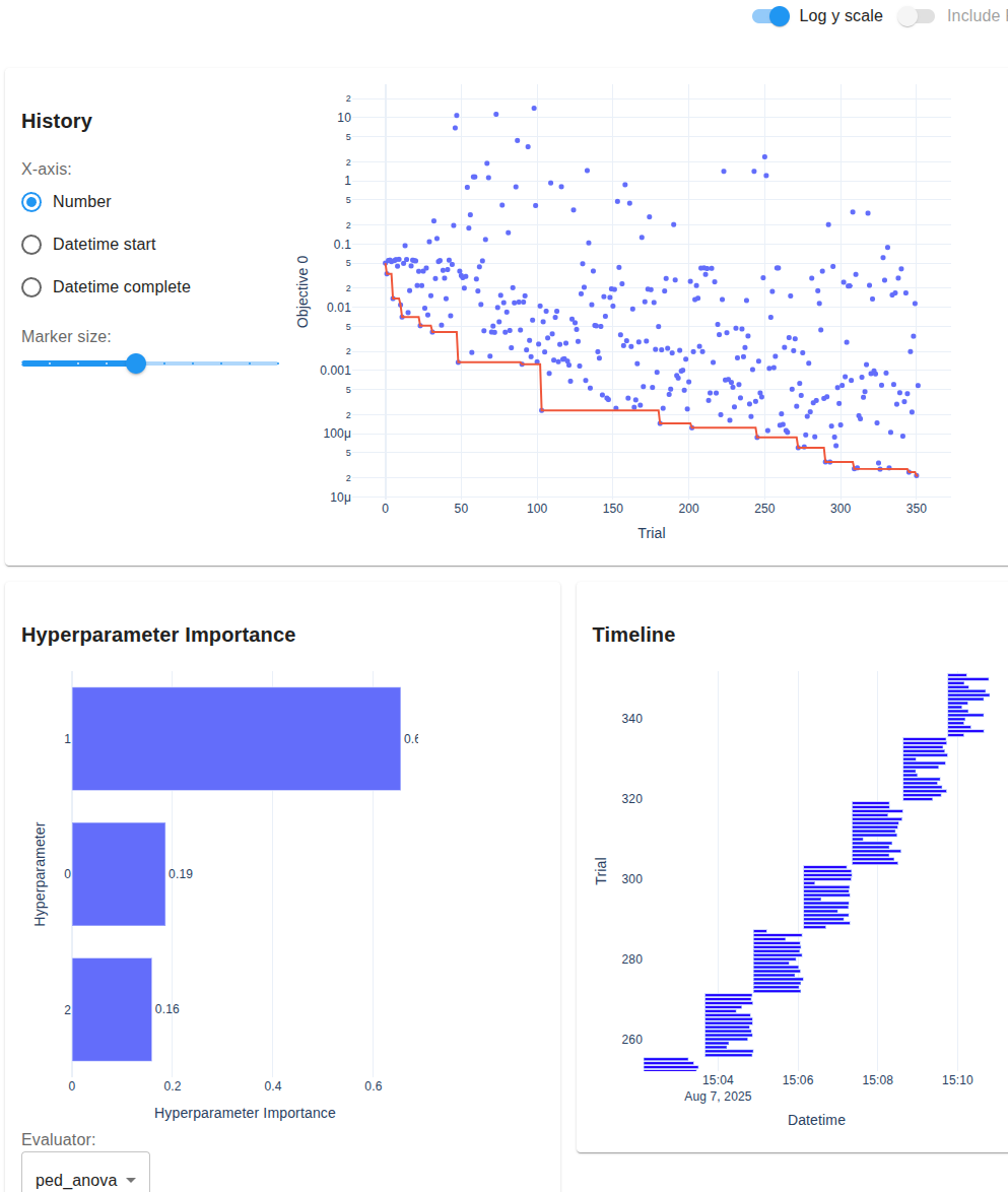
To use the Optuna dashboard:

Run pip install optuna-dashboard
Start the dashboard with optuna-dashboard journalMoran.log
Open http://127.0.0.1:8080/ in your browser

Explanation of Optimization Parameters

bounds Box boundaries for the parameters. This is an instance of scipy.optimize.Bounds.
popsize This is the population size used by the evolutionary algorithm, either Differential Evolution or CMA-ES.
- A larger popsize reduces the risk of getting stuck in local minima but makes convergence slower.
- For best performance, set popsize as a multiple of the number of parallel workers in fcmaes.evaluator.parallel.
- On a 16-core CPU, popsize = workers = 16 worked well in our tests and is a good starting point.
es (the optimization algorithm)
- fcmaes.de.DE (Differential Evolution) is a reliable default. Setting keep=20 makes the search broader. Use this mainly when you can only afford a limited number of evaluations.
- fcmaes.decpp.DE_C (C++ version) is a bit faster and supports providing an initial guess (x0), which is useful for improving an existing solution.
- fcmaes.cmaes.Cmaes and fcmaes.cmaescpp.ACMA_C are the Python and C++ versions of CMA-ES. They worked, but Differential Evolution performed slightly better for our case.
- If you have a good initial guess, setting a small input_sigma focuses the search.
- The other fcmaes algorithms with ask/tell support performed poorly for the Moran simulation. Only use them if you are sure they fit your use case.
terminate(fvals) This is an optional user-defined function. It decides when to stop based on the list of best function values from each iteration.

Alternative: Use minimize

If you do not need full control over the optimization loop, fcmaes provides a simpler option: minimize. Like fcmaes.evaluator.parallel, it has a workers parameter that defines how many Python processes are used. For the Moran simulation, these variants are relevant:

fcmaes.de.minimize: Differential Evolution, Python variant
fcmaes.cmaes.minimize: CMA-ES, Python variant

Warning: Avoid using the C++ variants fcmaes.decpp.minimize and fcmaes.cmaescpp.minimize for expensive simulations run from Python. These use C++ multithreading, which is limited by Python’s Global Interpreter Lock (GIL) and can lead to poor parallel performance. But you can use these variants in combination with the ask/tell interface.

fcmaes.bitecpp.minimize is very effective, but it does not have a workers parameter. Use it when the simulation itself is already parallelized.

In that case, the optimization loop becomes simpler:

    max_evaluations = 1200
    popsize = 16
    objective = journal_wrapper(wrapper(partial(objFunc2M, args)), bounds,
                        "journalMoran.log", "Moran", study_id=0, batch_size=popsize)
    result = fcmaes.de.minimize(objective, len(bounds.lb), bounds, workers=popsize, popsize=popsize, max_evaluations=max_evaluations)
    # use CMA-ES instead
    # result = fcmaes.cmaes.minimize(wrapper(partial(objFunc, args)), bounds, workers=popsize, popsize=popsize, max_evaluations=max_evaluations, input_sigma=0.5)
    # if you have a good initial guess
    # result = fcmaes.cmaes.minimize(wrapper(partial(objFunc, args)), bounds, workers=popsize, popsize=popsize, max_evaluations=max_evaluations, x0=guess, input_sigma=0.1)