fcmaes - a Python 3 gradient-free optimization library

Competing at ESAs Quantum Communications Constellations Challenge

This tutorial

Shows how to compete at an optimisation competition like Quantum Communications Constallations, which is part of the GECCO 2023 Space Optimisation Competition.
Shows how to utilize all CPU cores by parallelizing the optimisation process.
Introduces new parallel (meta-)algorithms aiming specifically to optimize the resulting pareto front.
Shows how to "speed up" the objective function computation by factor 30 with little effort re-implementing a few helper functions using numba and by switching to a faster graph representation.

Motivation

The Quantum Communications Constallations competition timeline was from 1 April until 30 June 2023. Most competitors struggled to come up with a reasonable solution for the given multi-objective task for several reasons:

The given objective function is expensive.
A fast re-implementation seems to be difficult - which is not the case as we will see below.
Existing Python libraries and algorithms like pygmo or pymoo NSGA II struggle to improve the resulting hypervolume above a certain threshold and don’t provide support for parallelization scaling well with the number of cores.

After reading this tutorial you should be able to improve your score significantly further.

Tutorial Code

The complete code corresponding to this tutorial is at quantumcomm.py This code uses spoc-2-quantum-communications-constellations-quantum-communications-constellatio_BpXhIVq.py as a basis, speeds up the objective function and adds the application of several optimisation algorithms.

Speedup using numba and igraph

The original code for the fitness function of the problem uses the networkx graph library implemented in python. This library should not be used to determine the average shortest path inside a time critical fitness function called millions times. Instead, for this purpose a faster alternative like igraph which wraps a C-based library should be applied. We can keep using networkx for all non time critical purposes like visualization. We have to adapt both graph construction and the shortest path computation. Note that we have omitted some checks present in the original, so we need to keep the original fitness for verification.

# computing the shortest path is much faster using igraph
# omits some checks
# use the original fitness to verify the pareto front

import igraph as ig

build_graph(self, ep_idx, pos, num_w1_sats, eta):
...
    adjmatrix, d_min = get_adjmatrix(pos, ep_idx, eta, num_w1_sats, self.LOS, N, self.eps_z, self.n_rovers)
    G = ig.Graph.Adjacency((adjmatrix > 0).tolist())
    G.es['weight'] = adjmatrix[adjmatrix.nonzero()]
    return G, adjmatrix, d_min


def average_shortest_path(self, G, src, dst):
    n_nodes = G.vcount()
    src0 = n_nodes - src - dst
    dst0 = n_nodes - dst
    sp = np.array(G.distances(list(range(src0, src0+src)), \
                              list(range(dst0, dst0+dst)), weights=G.es["weight"]))
    return np.mean(sp)

Even more important is to factor out other time critical functions performing operations on numba arrays to standalone functions outside the objects. These may then be annotated with '@njit()' using numba. Avoid non-numba nested loops at all cost in Python. Since the existing code already is based on numpy the adapted functions are very similar to the original version they replace:

from numba import njit
...
@njit()
def get_adjmatrix(pos, ep_idx, eta, num_w1_sats, LOS, N, eps_z, n_rovers):
    adjmatrix = np.zeros((N, N))
    d_min = np.inf
    for i in range(N):
        for j in range(i):
            # Ensure there is LOS
            los = line_of_sight(pos[i, ep_idx, :], pos[j, ep_idx, :])
            cos_theta_z = zenith_angle(pos[i, ep_idx, :], pos[j, ep_idx, :])
            if los >= LOS or cos_theta_z > 0:
                # Eta based on j because it is the destination satellite in the link
                eta_j = eta[0] if j < num_w1_sats else eta[1]
                adjmatrix[i,j], d_link = \
                    qkd_metric(N-i, pos[i, ep_idx, :], pos[j, ep_idx, :], cos_theta_z, eta_j, eps_z, n_rovers)
                if d_link < d_min:
                    d_min = d_link
                adjmatrix[j,i] = adjmatrix[i,j]
    return adjmatrix, d_min

These minor changes avoid the need to recode the original fitness using another programming language achieving an overall speedup of around factor 30. If we succeed in achieving an additional factor 12-15 using parallelization - which is possible using a modern 16 core CPU - this results in a quite significant overall speedup factor > 400.

During the Competition

Let us suppose it is end of June 2023, we want to improve our result before the competition ends. Team fcmaes is first with a score of -6399 (hypervolume = 0.6399), Team HRI is second with a score of -6382, team ML Actonauts - which will finally win - has not yet uploaded. So far this is what really happened at that time. Our best solution scores -6372 - stored in 'res/quantcomm_1_100_6372134.npz'. We would like to take the lead.

Applying a classical MO-algorithm: NSGA-II using simulated binary crossover and polynomial mutation.

Our first attempt is to apply fcmaes MO-optimisation using simulated binary crossover population update - see quantumcomm.py method 'mo_par'. Some features of this algorithm:

Parallel function evaluation.
Improvement of an existing pareto front
ask,tell interface.

This algorithm has a lot in common with classical NSGA-II with some tweaks regarding parallelization.

def mo_par():
    # inject an existing pareto front
    guess, _ = read_solution("res/quantcomm_1_100_6372134.npz")
    popsize = 512

    #  MOO optimizer
    es = mode.MODE(nobj, ncon, bounds, popsize = popsize, nsga_update=True)

    # use fcmaes parallel executor
    fit = parallel_mo(fitness, nobj+ncon, workers = mp.cpu_count())
    iters = 0
    stop = 0
    max_hv = 0
    time_0 = time.perf_counter()
    if not guess is None:
        es.set_guess(guess, fitness)

    while stop == 0 and iters < 100000:
        xs = es.ask()
        ys = fit(xs)
        es.tell(ys) # tell evaluated x
        iters += 1
        valid = [y[:2] for y in ys if np.less_equal(y , np.array([1.2, 1.4, 0, 0])).all()]
        hv = pg.hypervolume(valid).compute(ref_point)
        if hv > max_hv:
            max_hv = hv
        if hv > max_hv:
            logger.info(f'time: {dtime(time_0)} iter: {iters} hv: {hv * 10000}')
            np.savez_compressed("quantcomm_" + str(int(hv * 1000000)), xs=xs, ys=ys)
    fit.stop()
    return xs, ys

Together with our factor 30 speedup gained by numba and igraph (see last section) which allows us to use a large population size of 512, our 16 core CPU (AMD 7950x) is able to reach score -6398 after 80 minutes. But after that the algorithm got stuck. So close …

The code uses a new feature of fcmaes MO-optmization: Using 'set_guess' you now can define an initial population as guess - some pareto front you want to improve. The code also works with 'guess = None', although it needs more time. Using the ask/tell interface we can check the hypervolume each iteration and log/store improvements.

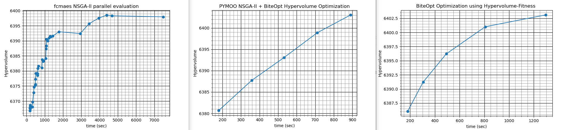
The left diagram shows the progress of this algorithm over time. To reach our goal we need to invent something new.

Applying alternative approaches

Below we will present two alternative approaches - developed after the competition - which get stuck at a much later point. As we can derive from the other two diagrams, these methods both can reach -6400 in a couple of minutes if initialized with our -6374 pareto front. If applied alternately, these methods finally reached a score of -6466.6.

Note, that only the Pymoo/BiteOpt approach shows scores for a 100-solutions pareto front. The results for the other two methods need first to be reduced to 100 solutions - we will show below how that works. This conversion leads to a slightly reduced score.

The tutorial code at quantumcomm.py is preconfigureed to reproduce these three diagrams for the three algorithms.

pymoo

Pymoo is a very popular optimisation library (nearly 2 million downloads) With pymoo parallelization works using the given objective function, but its overhead is so high that it slows down the computation instead of speeding it up.

from pymoo.core.problem import StarmapParallelization
from multiprocessing.pool import ThreadPool
...
pool = ThreadPool(mp.cpu_count())
runner = StarmapParallelization(pool.starmap)
problem = MyProblem(elementwise_runner=runner)

The speedup factor 30 we achieved in the previous section bites us, since it increases the relative overhead caused by 'StarmapParallelization'. We could start pymoo-NSGA-II manually in parallel and join the results - but this would most probably not result in a score better than -6400.

Why pymoo ?

fcmaes has its own MOO-algorithm optimized for parallelization, but we chose pymoo for this tutorial to show:

You can easily integrate algorithms from other libraries if they fit.
High algorithm overhead is less relevant for expensive fitness functions.
Bad scaling for parallelization doesn’t matter if you implement your own parallelization mechanism.

How to build your pareto front?

Last section we used the population maintained by the MOO algorithm to create the pareto front / check the hyper-volume. Usually this works very well, but not necessarily for a competition were we want to fine tune our result. When we inspect the left diagram above we see that the hyper-volume may drop slightly for the following generation. The new approach changes that using the following ideas:

Improve the pareto front iteratively, were each iteration improves the existing front by executing many optimisation runs in parallel.
The existing front is joined with all solutions of all these optimisations to generate the next pareto front.
Solutions are collected inside the fitness function independent of the actual population maintained by the pymoo optimizer.
These solutions are maintained for all parallel optimizers locally in their threads to minimize interprocess communication.
Only the pareto-front is stored to reduce the number of maintained solutions.
Only if the hyper-volume improves, the pareto front is shared globally via a managed multiprocessing dictionary.

After each iteration the pareto fronts for each optimisation is collected and joined with the previous result. One problem remains: The resulting pareto front may grow fast to more than 2000 solutions. Before we proceed with the next iteration, we need to reduce its size without harming its hyper-volume. Fortunately this is only a few lines of code using fcmaes - here fcmaes manages the parallelization and provides a well suited optimisation algorithm (BiteOpt).

# Uses https://github.com/avaneev/biteopt / parallel optimisation to find the best num solutions
# maximizing the pareto front

def reduce(xs, ys, num, evals = 50000, retries = mp.cpu_count()):
    if len(ys) <= num:
        return xs, ys
    bounds = Bounds([0]*num, [len(ys)-1E-9]*num) # select best num from xs, ys

    # selects 100 solutions and returns the negated pareto front of this selection
    def fit(x):
        selected = x.astype(int)
        ys_sel = ys[selected]
        hv = pg.hypervolume(ys_sel)
        return -hv.compute(ref_point) * 10000

    # parallel optimisation restart / retry
    res = fcmaes.retry.minimize(wrapper(fit),
                         bounds,
                         optimizer=Bite_cpp(evals),
                         num_retries=retries)

    selected = res.x.astype(int)
    return xs[selected], ys[selected]

Exercise: Try to apply a more classical OR approach (for instance using integer programming) and compare its performance and code size.

BiteOpt is hard to beat for this application. It requires multiple restarts which can be executed in parallel. Here is the rest of the code for the pymoo based optimisation. See 'pymoo_par' at quantumcomm.py for the complete code.

guess = None

class fitness_wrapper():

    def __init__(self,
                 pid,
                 xs_out,
                 ys_out
                ):
        self.max_hv = 0
        self.xs = []
        self.ys = []
        self.count = 1
        self.evals = 0
        self.pid = pid
        self.xs_out = xs_out
        self.ys_out = ys_out

    # fitness accumulates valid solutions and monitors their hypervolume
    def __call__(self, x):
        y = fitness(x)
        self.evals += 1
        # add only valid solutions
        if np.amax(y[2:]) <= 0 and np.less_equal(y[:2], ref_point).all() :
            # exclude constraint values because solution is valid
            self.ys.append(y[:2])
            self.xs.append(x)
        if len(self.ys) >= 2*popsize:
            self.count += 1
            # reduce to pareto front
            xs, ys = moretry.pareto(np.array(self.xs), np.array(self.ys))
            self.xs, self.ys = list(xs), list(ys)
            hv = pg.hypervolume(self.ys).compute(ref_point)
            # significant improvement: register solutions at managed dicts
            if hv > self.max_hv * 1.0001:
                self.max_hv = hv
                self.xs_out[self.pid] = self.xs
                self.ys_out[self.pid] = self.ys
                logger.info(f'time: {dtime(time_0)} ev: {self.evals} hv: {hv * 10000} n: {len(ys)}')
        return y

class OptPymoo(object):

    def eval_loop(self, workers=mp.cpu_count()):
        xs = guess
        for i in range(1, 1000):
            xs, ys = self.eval(i, xs, workers)
        return xs, ys

    def eval(self, i, guess, workers):
        manager = Manager()
        xs_out = manager.dict() # for inter process communication
        ys_out = manager.dict() # collects solutions generated in the sub processes
        fits = [fitness_wrapper(pid, xs_out, ys_out) for pid in range(workers)]
        proc=[mp.Process(target=self.optimize, args=(guess, fits[pid], pid)) for pid in range(workers)]
        [p.start() for p in proc] # spawn NSGAII optimisation workers
        [p.join() for p in proc]
        # join collected solutions, we ignore the pymoo optimisation result
        xs = np.array(list(chain.from_iterable(xs_out.values())))
        ys = np.array(list(chain.from_iterable(ys_out.values())))
        xs, ys = moretry.pareto(xs, ys)
        if len(ys) > target_num:
            xs, ys = reduce(xs, ys, target_num)
        hv = int(pg.hypervolume(ys).compute(ref_point) * 10000000)
        np.savez_compressed("quantcomm_" + str(i) + "_" + str(len(ys)) +
                            "_" + str(hv), xs=xs, ys=ys)
        return xs, ys

    def optimize(self, guess, fit, pid):

        class MyProblem(ElementwiseProblem):

            def __init__(self, **kwargs):
                super().__init__(n_var=dim,
                                 n_obj=nobj,
                                 n_constr=ncon,
                                 xl=np.array(bounds.lb),
                                 xu=np.array(bounds.ub), **kwargs)

            def _evaluate(self, x, out, *args, **kwargs):
                y = fit(x)
                out["F"] = y[:nobj]
                out["G"] = y[nobj:]

        problem = MyProblem()
        algorithm = NSGA2(
            pop_size=popsize,
            n_offsprings=10,
            sampling=FloatRandomSampling() if guess is None else guess,
            crossover=SBX(prob=0.9, eta=15), # simulated binary crossover
            mutation=PM(eta=20), # polynomial mutation
            eliminate_duplicates=True,
        )
        algorithm = AdaptiveEpsilonConstraintHandling(algorithm, perc_eps_until=0.5)
        minimize(problem, algorithm, get_termination("n_eval", n_eval), verbose=False, seed=pid*677)

opt = OptPymoo()
return opt.eval_loop()

The performance of the pymoo based hypervolume optimisation executed using a AMD 7950x 16 core CPU is shown below.

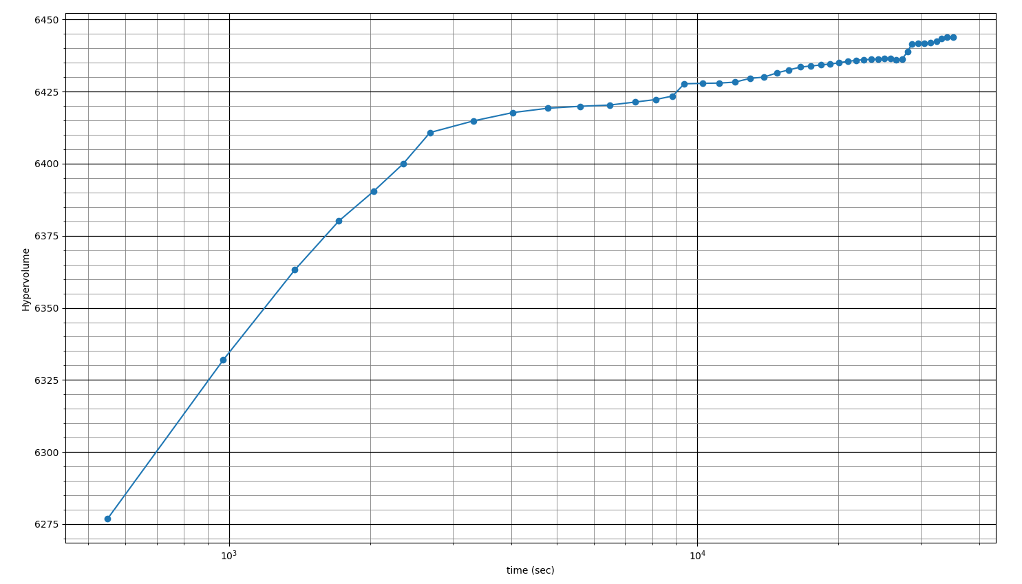
As we can see, it would have been sufficient to achieve a competitive score if run overnight, even if it starts with an empty guess. Note that we apply 'AdaptiveEpsilonConstraintHandling' to improve constraint handling.

Single Objective optimisation of the Pareto Front

Do we need MOO-algorithms at all? Why not divide the problem in many sub-problems each to be solved by a single objective optimizer? But how can we do that and what should be the single objective ? See https://esa.github.io/pygmo2/mo_utils.html 'pygmo.decompose_objectives' to get an idea what is usually done: You may compute a weighted sum of the objectives and the decomposition means choosing different weights.

Exercise: Since this is an ESA challenge, pygmo is already imported. Try applying 'pygmo.decompose_objectives' to improve an existing pareto front using the single objective optimizer of your choice.

Here we will choose another idea:

Decomposition is done related to the different solutions in the pareto front. For each solution as guess we perform a separate optimisation.
As in the previous section optimisations are performed in parallel, and we divide the whole process into a sequence of iterations.
As single objective we choose directly the hyper-volume of the whole front - where the solution we improve is replaced by the current solutions checked by the algorithm.
As for the reduction algorithm above we use the BiteOpt algorithm as single objective optimizer.
The current pareto front is shared between processes using a managed list. As soon as there is an improvement, the corresponding solution is replaced in the shared pareto front.

    # hypervolume replacing one solution of the pareto front
    def fit_hyper(i, ys, x):
        y = fitness(x)
        c = sum([10000 + c for c in y[2:] if c > 0])
        if c > 0: # constraint violation
            return c
        if pg.pareto_dominance(y[:2], ref_point):
            ys[i] = y[:2]
            return -pg.hypervolume(ys).compute(ref_point) * 10000
        else:
            return 0

    # parallel optimisation of the whole pareto front
    class OptSo(object):

        def __init__(self,
                     max_evals,
                     xs,
                     ys
                    ):
            self.max_evals = max_evals
            self.manager = Manager()
            self.ys = self.manager.list(ys)
            self.ys0 = list(ys)
            self.xs = self.manager.list(xs)
            self.min_ys = np.amin(ys, axis=0)
            self.count = mp.RawValue(ct.c_int, 0)
            self.mutex = mp.Lock()
            self.n = len(ys)

        def incr(self):
            with self.mutex:
                next = self.count.value
                self.count.value += 1
                return next

        def eval(self, workers=mp.cpu_count()):
            proc=[mp.Process(target=self.eval_loop) for pid in range(workers)]
            [p.start() for p in proc]
            [p.join() for p in proc]
            return np.array(self.xs), np.array(self.ys)

        def eval_loop(self):
            while True:
                i = self.incr()
                if i >= self.n:
                    return
                logger.info(f'optimizing solution {i}')
                fit = wrapper(partial(fit_hyper, i, list(self.ys)))
                x0 = self.xs[i]
                ret = bitecpp.minimize(fit, bounds, x0, max_evaluations = self.max_evals)
                if ret.fun < 0: # no constraint violation?
                    y = fitness(ret.x)[:2]
                    self.ys[i] = y
                    self.xs[i] = ret.x

    def opt_so(max_evals, xs, ys, workers=mp.cpu_count()):
        eval = OptSo(max_evals, xs, ys)
        return eval.eval(workers)

    max_evals = 2000

    # initialization with a given pareto front
    xs, ys = read_solution("res/quantcomm_1_100_6372134.npz") # inject an existing pareto front

    last_xs = []
    last_ys = []
    for i in range(1, 1000):
        xs, ys = opt_so(max_evals, xs, ys)
        xs, ys = moretry.pareto(np.array(list(xs) + last_xs),
                                    np.array(list(ys) + last_ys))
        if len(ys) > target_num:
            xs, ys = reduce(xs, ys, target_num)
        hv = int(pg.hypervolume(ys).compute(ref_point) * 10000000)

        np.savez_compressed("quantcomm_" + str(i) + "_" + str(len(ys)) + "_"
                            + str(max_evals) + "_" + str(hv), xs=xs, ys=ys)
        last_xs = list(xs)
        last_ys = list(ys)

    return xs

As we can see below, the performance of the algorithm - using a 16 core AMD 5950x CPU - is comparable to the pymoo approach shown above. Both methods struggle with the score -6450 barrier. Note, that we have to maintain a larger pareto front here - which means the final score using a 100-solution front will be slightly lower.

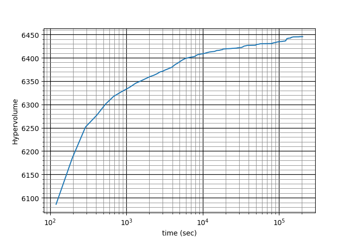
The final score achieved by team fcmaes (after the competition) by alternating between both methods is -6466.6.

Quality Diversity optimisation

Applying a QD algorithm helps us to visualize the whole objective / constraint space. We seed the ND-optimizer with a pareto front generated by one of the other methods shown above, since these are more effective in optimizing the pareto front. For less complex tasks no other optimizer is required.

Analyzing the resulting diagrams we learn:

There is a tradeoff between constraint 1 (surface cover / rover distance) values and the objectives. Tightening constraint 1 leads to slightly worse objective values. Surprisingly relaxing of constraint 1 does not help the objectives at all.
Constraint 2 (satellite distance) seems unrelated to the objectives. Good solutions tend to have a much larger satellite distance than required by the constraint.

So you know that you don’t have to fear satellite collisions at all - and may even drop this constraint. And that you can increase the covered surface by investing more. The left diagram even tells you how much you need to invest where to cover a certain area. And that the required minimum (3000km) is covered even by the cheapest solutions.

Exercise: Try to derive these facts from the pareto front or its hyper-volume alone. Hint: Check the constraint values of the pareto solutions. Do these provide sufficient information?

For real world problems you probably don’t want to base your decision only on the pareto front, specially if:

The model for the objectives / constraints has limited accuracy.
There are good solutions slightly violating some constraints, or which allow to tighten some constraints further.

Maybe ESA could consider to add a QD-score component to the overall score of a future optimisation challenge to cover the "diversity" aspect.

See quantumcomm.py function 'nd_optimize' to see the code corresponding to this section. Visualizing the resulting QD-archive produced by this code we get:

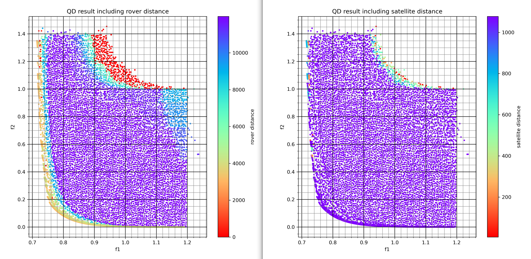
The left diagram shows rover distance values as colors, the right one satellite distance values.

def mo_to_qd(y):
    f1, f2, c1, c2 = y
    # weight the objectives and constraints
    return f1/0.5 + f2/1.4 + c1/3000 + c2/50, \
           np.minimum(ref_point, np.array([f1, f2])) # use the objectives as descriptive space

def qd_fun(x):
    return mo_to_qd(fitness(x)) # convert the MO result into a QD result

def get_arch(qd_bounds, niche_num, samples_per_niche):
    xs, _ = read_solution("res/quantcomm_1_100_6372134.npz") # inject an existing pareto front
    arch = mapelites.empty_archive(dim, qd_bounds, niche_num, samples_per_niche)
    mapelites.update_archive(arch, xs, qd_fun)
    return arch

def nd_par(niche_num = 10000):
    udp = constellation_udp()
    ubs = udp.get_bounds()
    qd_bounds = Bounds([0.7, 0.], [1.2, 1.4])
    samples_per_niche = 20
    arch = get_arch(qd_bounds, niche_num, samples_per_niche)
    opt_params0 = {'solver':'elites', 'popsize':100, 'use':2}
    opt_params1 = {'solver':'CRMFNES_CPP', 'max_evals':2000, 'popsize':32, 'stall_criterion':3}
    archive = diversifier.minimize(
         mapelites.wrapper(qd_fun, 2, interval=10000, save_interval=100000),
         bounds, qd_bounds,
         workers = 32, opt_params=[opt_params0, opt_params1], archive = arch,
         niche_num = niche_num, samples_per_niche = samples_per_niche,
         max_evals = 1000000)

    print('final archive:', archive.info())
    archive.save('final archive')

As QD-algorithm we use is a - configurable - combination of Map-Elites using Voronoi tessellation with CR-FM-NES. See Quality Diversity for a detailed description of this algorithm which generalizes CMA-ME and CVT MAP-Elites.

Note that for QD optimization we may use a weighted sum for the objectives and even the constraints without loosing diversity. Using both objectives as descriptive space ensures that we still find solutions for different combinations of the objective values. The weighted sum here serves two purposes:

It helps to identify the most "interesting" solution insides its niche: The one which doesn’t violate the constraint.
It "drives" the search into the "right" direction when starting from a niche: Improved objective and constraint values.