

Quality-Diversity applied to expensive simulations
This tutorial
-
Explains how to apply QD algorithms (Quality Diversity) to expensive simulations in power plant design, biochemical reactions, stock trading, water management, and car design and crash simulation.
-
Compares different configurations and improvement emitters.
-
Shows how to "zoom in" on QD archives and how to combine QD algorithms with MO algorithms.
Remark
If you just want to experiment with QD algorithms, start with the simple example arm.py, which simulates a planar robot arm. Change the parameters or algorithms to get a feel for how they behave.
Motivation
In MapElites.adoc we looked at QD optimization from the perspective of an extremely hard problem to understand its limits. We found that QD methods are still applicable even on very rugged solution landscapes such as Cassini2, provided that:

-
We fully use the parallelism of modern many-core CPUs.
-
We combine MAP-Elites with evolutionary algorithms such as CMA-ES and CR-FM-NES.
These methods need many fitness evaluations. That raises an obvious question: what happens when each evaluation is expensive because it runs a detailed simulation?
Technical simulations are usually used to understand how input parameters affect system behavior and to identify good parameter settings. In practice, "good" rarely means only one objective. Constraints matter too, and some of them may be flexible. If a small relaxation of a constraint leads to a large improvement, we may decide that the tradeoff is acceptable. For that reason, it is often not a good idea to encode every constraint directly into the optimization problem from the start. It is usually better to explore the design space first and decide later which constraints are acceptable. The same applies to multiple objectives. We can postpone the choice of their weights until we have seen the available tradeoffs.
This means moving away from the usual idea of a single objective, or even a fixed set of objectives, as required by standard optimization algorithms. One option would be to sweep the parameter space with a grid or random samples. That can work for small problems, but it breaks down as the number of decision variables grows. More importantly, the tessellation should usually not be based on the input parameters. It should be based on derived properties that describe the behavior of the simulation. For example:
Imagine a power plant simulation where we care about efficiency, defined as power divided by heat. Then the tessellation should be based on the derived properties power and heat, not on the input parameters. This leads to two questions:
-
How do we obtain the behavior values, and how should we tessellate them?
-
How do we generate the parameter settings we want to evaluate?
The first question is straightforward. Behavior is observable during the simulation, so the fitness function can return an additional behavior vector. CVT Map Elites proposes a Voronoi tessellation that can be implemented efficiently with sklearn.neighbors.KDTree and sklearn.cluster.KMeans. We tessellate the behavior space into niches and store the elite of each niche, meaning the fittest solution found there, in a QD archive. Building the KDTree can be expensive if we use 10000 or more niches, but caching the niche means helps. If the behavior space is normalized to [0,1] in each dimension, these cached means can even be shared across problems as long as the number of dimensions and niches stays the same. fcmaes does this caching automatically.
The second question is harder. We want to do better than random sampling and focus on interesting parts of the solution space. So we reintroduce an objective, not to find one global optimum, but to define what "interesting" means. There are different ways to handle multiple objectives. For example, we could use a weighted sum as the fitness objective and still preserve diversity by using the individual objectives as behavior dimensions. In the rest of this tutorial we focus on the simpler case of a single fitness objective. In the power plant example, "interesting" means "efficient", so efficiency becomes the fitness objective.
When should you consider using fcmaes for QD?
When does fcmaes make sense for simulation analysis with QD, and why? The fcmaes QD algorithms support parallel fitness and behavior evaluations that all share one QD archive. In many cases, this scales much better than parallelizing the simulation itself. The implementation builds on ideas from fcmaes parallel retry, which also uses a solution archive shared by parallel optimization processes.
Consider fcmaes if:
-
Your simulation is expensive and your CPU or CPUs have many cores.
-
You do not want to parallelize the simulation itself, or parallelizing it gives poor scaling.
-
Your simulation can be called through a Python or C/C++ API. For C/C++ APIs, create a Python wrapper with ctypes as done in some of the examples here. Avoid launching simulations as separate executables. The overhead is often underestimated. See Evolving many-objective water management to exploit exascale computing, which discusses the Lower Rio Grande Valley (LRGV) water management problem. As shown below, a regular many-core CPU is already sufficient for that problem.
You can also run several QD optimizations on different CPUs and merge the resulting archives later to improve behavior-space coverage.
Exploration versus Exploitation
In QD algorithms, the way new candidates are generated depends on the algorithm settings. fcmaes gives you a lot of control here. These settings balance exploration against exploitation, and the best balance depends on the problem. The goal is strong exploitation so we do not miss very good solutions, while still maintaining enough exploration to cover the behavior space. Since exploration is usually the easier part, fcmaes puts more emphasis on exploitation.
Ease of Use
You may not want to tune a large set of QD parameters. You may just want a reasonable result out of the box. fcmaes provides a default setup that runs both MAP-Elites and an improvement emitter in parallel, and this works well in most cases. You can still adapt the population or batch size, but for many applications the default already performs well. MO algorithms are usually more sensitive in this regard.
Customization
If you do want to tune the algorithm, fcmaes offers many options:
-
You can choose the base algorithm for the improvement emitter. Current options are CMA-ES, CR-FM-NES, DE, PGPE, and BiteOpt. This matters because CMA-ES, although popular, is not the best choice for every application.
-
Improvement emitters can be chained. See elitescass2.py, where such a sequence gives the best configuration.
-
Mixing MAP-Elites with an improvement emitter is not new, but fcmaes assigns separate parallel processes to each task while they share one archive. By default, half of the processes run MAP-Elites, but you can change that. For example, on a 16-core CPU with hyperthreading you could assign 12 processes to MAP-Elites and 20 to the configured improvement emitter.
-
You can tune many parameters of the selected improvement emitter.
Related work
qdo_yahpo provides a framework for testing QD hyperparameter optimization. It uses a surrogate model that can be executed single-threaded, which makes parallel testing easy. We applied these benchmarks to fcmaes diversifier in yahpo.py.
The main differences are:
-
fcmaes uses a QD archive shared between parallel processes, each running either CVT MAP-Elites or an improvement emitter.
-
fcmaes uses Voronoi tessellation, as described in CVT MAP-Elites.
-
Instead of a Gaussian distribution, fcmaes can use simulated binary crossover plus polynomial mutation, as in NSGA-II.
-
The number of parallel processes assigned to each emitter is configurable.
-
Improvement emitters do not have to use CMA-ES. Current alternatives are CR-FM-NES, DE, BiteOpt, and PGPE.
-
Improvement emitters can be chained, for example DE → CMA, where the later emitter is initialized with the solution from the earlier one. This helps on extremely rugged fitness landscapes.
-
Improvement emitters are initialized with a random solution instead of a niche elite. This seems to work better.
Being able to choose the improvement-emitter algorithm is important, and the fcmaes diversifier meta-algorithm supports that directly. The problems discussed here work best with either CR-FM-NES or CMA-ES as the emitter. In MapElites.adoc, which applies the fcmaes diversifier to a space mission design problem through elitescass2.py, the best choice is a DE → CMA-ES sequence. In Scheduling.adoc (section QD update) it is BiteOpt. See also https://github.com/google/evojax/pull/52, where I created a PR for EvoJax that introduces the same idea in the machine learning domain.
fcmaes diversifier also performs very well on QD hyperparameter optimization, although a direct comparison is difficult because fcmaes uses Voronoi tessellation while qdo_yahpo uses a grid.
If a surrogate model is available, as in yahpo.py, parallelization is much easier because there is no GPU bottleneck. Without a surrogate, hyperparameter optimization often depends on a GPU or TPU that cannot easily be shared, which usually limits optimization to one thread per device.
Powerplant Simulation
The complete code for this example is here: powerplant.py. PowerPlant.adoc explains the single-objective and multi-objective variants. Here we extend the same example with QD methods.
The power plant simulation is based on tespy, a Python framework for thermal engineering systems. We vary the pressure at two extraction connections. These two pressures are the decision variables. After each simulation run, we divide power by heat to compute the efficiency that we want to maximize.
    def calculate_efficiency(self, x):
        # set extraction pressure
        self.nw.get_conn('extraction1').set_attr(p=x[0])
        self.nw.get_conn('extraction2').set_attr(p=x[1])

        self.nw.solve('design')
        ...
        return self.nw.busses['power'].P.val / self.nw.busses['heat'].P.val

    def calculate_qd(self, x):
        y = self.calculate_efficiency(x)
        desc = [self.nw.busses['power'].P.val, self.nw.busses['heat'].P.val]
        return y, desc
The QD behavior vector desc stores power and heat separately. Note that calculate_qd is protected by with threadpoolctl.threadpool_limits(limits=1, user_api="blas") so the simulation runs single-threaded. That avoids interference with the parallel optimization.
def run_diversifier():
    class qd_problem():

        def __init__(self):
            self.dim = 2
            self.qd_dim = 2
            self.bounds = Bounds([1]*self.dim, [40]*self.dim)
            self.qd_bounds = Bounds([2.2E8, 5E8], [2.8E8, 6.3E8])
            self.local = threading.local()

        def get_model(self):
            if not hasattr(self.local, 'model'):
                self.create_model()
            return self.local.model

        def create_model(self):
            self.local.model = PowerPlant()

        def efficiency(self, x):
            try:
                with threadpoolctl.threadpool_limits(limits=1, user_api="blas"):
                    eff, desc = self.get_model().calculate_qd(x)
                if not np.isfinite(eff): # model gets corrupted in case of an error
                    self.create_model() # we need to recreate the model
                    return 0, self.qd_bounds.lb
                return eff, desc
            except Exception as ex:
                return 0, self.qd_bounds.lb

        def qd_fitness(self, x):
            y, desc = self.efficiency(x)
            return 1-y, desc
The QD optimization is executed with diversifier.minimize. It runs MAP-Elites ('solver':'elites') and a CMA-ES improvement emitter ('solver':'CMA_CPP') in parallel, with half of the available threads assigned to each. qd_bounds normalizes the behavior values. max_evals=25600 limits the total number of fitness evaluations, while 'max_evals':200 limits one improvement-emitter run. In this example, CMA-ES is the best emitter base algorithm. That is not the case for most of the other simulation-based problems discussed later.
    problem = qd_problem()
    name = 'powerplant2'
    opt_params0 = {'solver':'elites', 'popsize':128}
    opt_params1 = {'solver':'CMA_CPP', 'max_evals':200, 'popsize':16, 'stall_criterion':3}
    archive = diversifier.minimize(
         mapelites.wrapper(problem.qd_fitness, 2, interval=1000), problem.bounds, problem.qd_bounds, opt_params=[opt_params0, opt_params1], max_evals=25600)
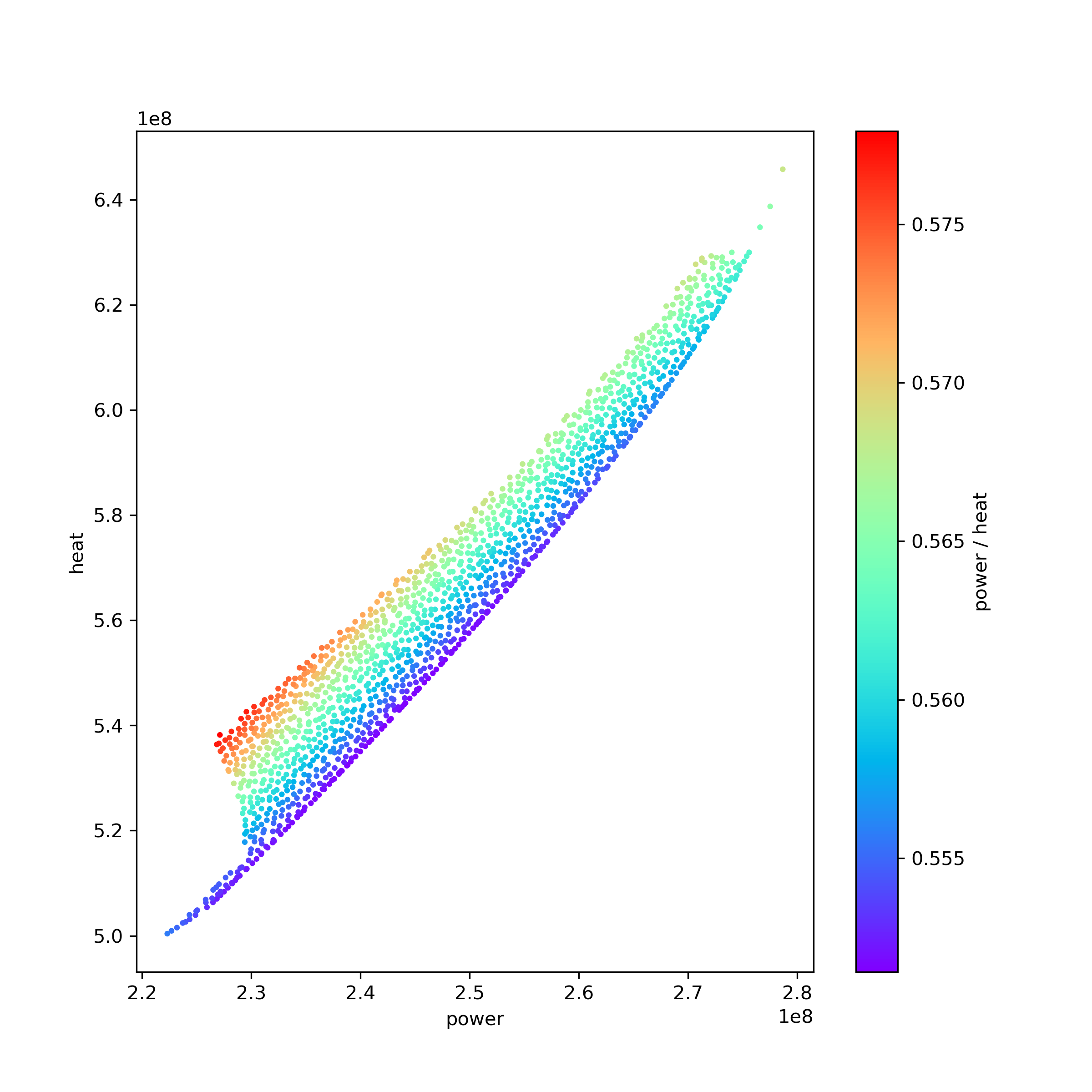
The resulting diagram shows how efficiency is distributed across different power and heat values. It becomes easy to identify the most efficient solutions for specific power and heat limits. Because fcmaes can store and reload the QD archive, you can make these decisions later in a separate analysis step. You can also restart the optimization from a stored archive with different optimization parameters. It is even possible to change the number of niches or the definition of the behavior vector in between, although that requires recomputing fitness values for the stored solutions.
Biochemical Reactions
The complete code for this example is here: vilar.py. Sweep.adoc explains the single-objective and multi-objective versions. Here we add QD methods.
In Mechanisms of noise-resistance in genetic oscillators, Jose M. G. Vilar introduced a biochemical model of a circadian clock that lets organisms keep an internal sense of daily time. The model can be simulated with GillesPy2; see VilarOscillator.py. The Vilar model has 15 parameters, and we want to answer these questions:
-
Does the oscillating behavior depend on specific parameter settings?
-
Can we find parameter settings that degrade the oscillation?
-
Or does the model show self-regulating behavior that preserves a steady oscillation?
We use scipy’s argrelextrema to identify the maxima of species R. Then we compute the standard deviation of the amplitudes and of the distances between peaks. Small values for these standard deviations indicate a steady oscillation, so we use them as objectives. ws = sdev_peak_dist/3.0 + sdev_amp/30.0, the normalized weighted sum of these standard deviations, serves as the fitness value. We also include the frequency in the behavior vector to increase diversification.
    class nd_problem():

        def __init__(self):
            self.bounds = get_bounds(VilarOscillator(), 100)
            self.qd_bounds = Bounds([0, 30, .035], [3, 300, .050])
            self.qd_dim = 3
            self.dim = len(self.bounds.ub)

        def fitness(self, x):
            with threadpoolctl.threadpool_limits(limits=1, user_api="blas"):
                model = VilarOscillator()
                set_params(model, x)
                res = model.run(algorithm = "SSA")
                R = res['R'] # time series for R
                r_mean = np.mean(R)
                r_over = np.array(np.fromiter((r for r in R if r > r_mean), dtype=float))
                ilocs_max = argrelextrema(r_over, np.greater_equal, order=3)[0]
                freq = len(ilocs_max) / len(R)
                peak_dists = np.array(np.fromiter((ilocs_max[i] - ilocs_max[i-1] for i in range(1, len(ilocs_max))), dtype=float))
                sdev_peak_dist = np.std(peak_dists)
                peaks = (r_over - r_mean)[ilocs_max]
                sdev_amp = np.std(peaks)
                ws = sdev_peak_dist/3.0 + sdev_amp/30.0 # weighted sum
                return ws, np.array([sdev_peak_dist, sdev_amp, freq])
This time we use CR-FM-NES as the base algorithm for the improvement emitter ('solver':'CRMFNES_CPP') and run it in parallel with MAP-Elites ('solver':'elites'). We choose a small population size because the simulation is expensive. Even with parallelization, we reach only about 8 simulations per second.
    problem = nd_problem()
    opt_params0 = {'solver':'elites', 'popsize':8}
    opt_params1 = {'solver':'CRMFNES_CPP', 'max_evals':200, 'popsize':16, 'stall_criterion':3}
    archive = diversifier.minimize(
         mapelites.wrapper(problem.fitness, problem.qd_dim, interval=100, save_interval=4000),
         problem.bounds, problem.qd_bounds, opt_params=[opt_params0, opt_params1], max_evals=12800)
    print("final archive: " + archive.info())
    archive.save("vilar_nd")
    plot_archive(archive)
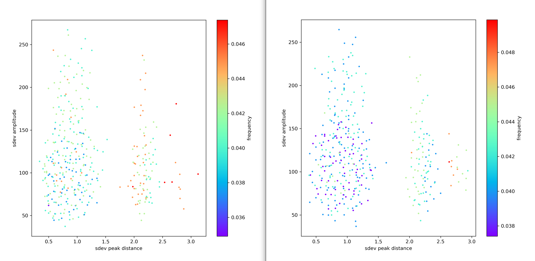
The resulting diagram also includes a second run where we maximize the objective ws = 2 - (sdev_peak_dist/3.0 + sdev_amp/30.0). Both diagrams look quite similar, which suggests that the objective plays only a small role here.
Stock Trade Simulation
The complete code for this example is here: crypto.py. CryptoTrading.adoc explains the single-objective and multi-objective versions. Here we add QD methods.
When we optimize a trading strategy on historical data, the main risk is overfitting to the past. The example already reduces that risk by optimizing ROI (return on investment) across 4 tickers and using the geometric mean ROI as fitness. This ROI is normalized against the HODL ROI, meaning the return we would get by buying and holding the entire time. We can now use the 4 normalized ROI factors as the behavior vector and generate a diverse set of solutions.
    def ndfun(self, x):
        y, factors, _ = self.fun(x)
        return 5+y, factors # we need positive y values for tracking QD-Score
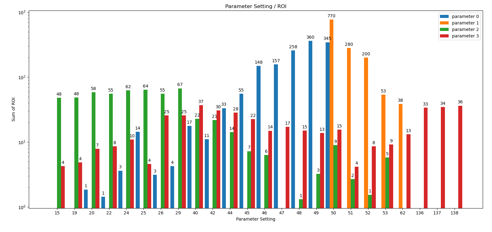
Once we have this archive of diverse solutions, we can count how often each parameter value occurs.
    ...
    bounds = Bounds([20,50,10,10], [50,100,200,200])
    qd_dim = 4
    qd_bounds = Bounds([0]*ddim, [4]*ddim)
    niche_num = 1000
    fit = fitness(tickers, start, end, None)
    opt_params0 = {'solver':'elites', 'popsize':100}
    opt_params1 = {'solver':'CMA_CPP', 'max_evals':10000, 'popsize':16, 'stall_criterion':3}
    archive = diversifier.minimize(
         mapelites.wrapper(fit.ndfun, qd_dim, interval=10000, save_interval=100000000),
         bounds, qd_bounds, opt_params=[opt_params0, opt_params1], max_evals=4000000)
    print("final archive: " + archive.info())
    archive.save("crypto_min_cma")

    ysi = archive.argsort()
    ys = archive.get_ys()[ysi]
    ds = archive.get_ds()[ysi]
    xs = archive.get_xs()[ysi]
    occupied = (ys < np.inf)

    for i, (y, d, x) in enumerate(zip(ys[occupied], ds[occupied], xs[occupied])):
        print(str(i+1) + ": y " + str(round(5-y,2)) +
              " fac " + str([round(di,2) for di in d]) +
              " x = " + str([int(xi) for xi in x]))
This gives us a more reliable indicator of which parameter values work well:
Water Resource Management
HBV Rainfall-Runoff Model
The complete code for this example is here: hbv.py. Water.adoc explains the multi-objective version. Here we add QD methods.
The rainfall-runoff multi-objective problem, discussed in Evolutionary multiobjective optimization in water resources, has three main routines:
-
snow accumulation and melt
-
soil moisture accounting
-
transformation of the linear outflow from two sub-basins
The model has 14 real-valued decision variables that must be calibrated. This is a real-world problem. Its multi-objective formulation was used to calibrate the HBV model for the Williams River in West Virginia, United States.
For QD, we use a weighted sum of the four objectives as fitness. The same four objectives form the behavior vector.
class hbv(object):
    ...
    def qd_fitness(self, x):
        y = self.__call__(x)
        b = y.copy()
        y = (y - self.qd_bounds.lb) / (self.qd_bounds.ub - self.qd_bounds.lb)
        ws = sum(y)
        return ws, b

def optimize_qd():
    problem = hbv()
    problem.qd_dim = 4
    problem.qd_bounds = Bounds([0.2, 0.7, 0, 0], [0.6, 1.3, 0.18, 0.6])
    opt_params0 = {'solver':'elites', 'popsize':64}
    opt_params1 = {'solver':'CRMFNES_CPP', 'max_evals':4000, 'popsize':32, 'stall_criterion':3}
    archive = diversifier.minimize(
         mapelites.wrapper(problem.qd_fitness, problem.qd_dim, interval=200000, save_interval=5000000),
         problem.bounds, problem.qd_bounds, opt_params=[opt_params0, opt_params1], max_evals=12000000)
    print('final archive:', archive.info())
    archive.save('hbv_qd')
Again, CR-FM-NES ('solver':'CRMFNES_CPP') works better than CMA-ES as the improvement-emitter base algorithm for this problem. Combined with MAP-Elites ('solver':'elites'), it produces the following result:
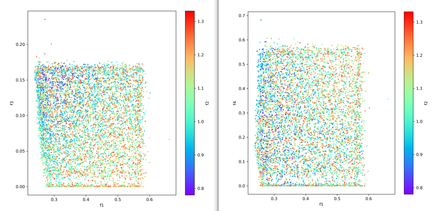
Since there are four objectives, each diagram shows three of them.
Lower Rio Grande Valley (LRGV) problem
The complete code for this example is here: lrgv.py. See also Water.adoc.
The Lower Rio Grande Valley (LRGV) framework models a risk-based water supply portfolio problem. A single city must choose an efficient mix of market-based sources and traditional reservoir sources while minimizing the risk of not having enough water available when needed. An option-based market lets the city secure water later at a fixed price by paying an option price in advance.
We forked the original code at https://github.com/dietmarwo/LRGV so it can be called from Python and made it reentrant. That greatly increases the number of simulations we can execute per second, so running 400000 fitness evaluations becomes easy.
We configure the framework with five objectives:
-
minimize water supply costs
-
maximize the reliability of meeting demands
-
minimize surplus water
-
minimize dropped or unused water transfers
-
minimize the number of leases required over a 10-year planning horizon
For QD, we use a weighted sum of these five objectives as the fitness value. The behavior vector contains the five objectives themselves.
class lrgv(object):
...
    def qd_fitness(self, x):
        y = self.__call__(x)
        b = y[:nobj].copy()
        constr = np.maximum(y[nobj:], 0) # we are only interested in constraint violations
        c =  np.amax(constr)
        if c > 0.001: c += 10
        y = (y[:nobj] - self.qd_bounds.lb) / (self.qd_bounds.ub - self.qd_bounds.lb)
        ws = sum(y) + c
        return ws, b

def optimize_qd():
    problem = lrgv()
    problem.qd_dim = 5
    problem.qd_bounds = Bounds([0.85E7, -1, 10000, 0, 0], [1.4E7, -0.985, 65000, 65000, 10])
    name = 'lrgv_qd'
    opt_params0 = {'solver':'elites', 'popsize':32}
    opt_params1 = {'solver':'CRMFNES_CPP', 'max_evals':400, 'popsize':16, 'stall_criterion':3}
    archive = diversifier.minimize(
         mapelites.wrapper(problem.qd_fitness, problem.qd_dim, interval=1000, save_interval=20000),
         problem.bounds, problem.qd_bounds, opt_params=[opt_params0, opt_params1], max_evals=400000)

    print('final archive:', archive.info())
    archive.save(name)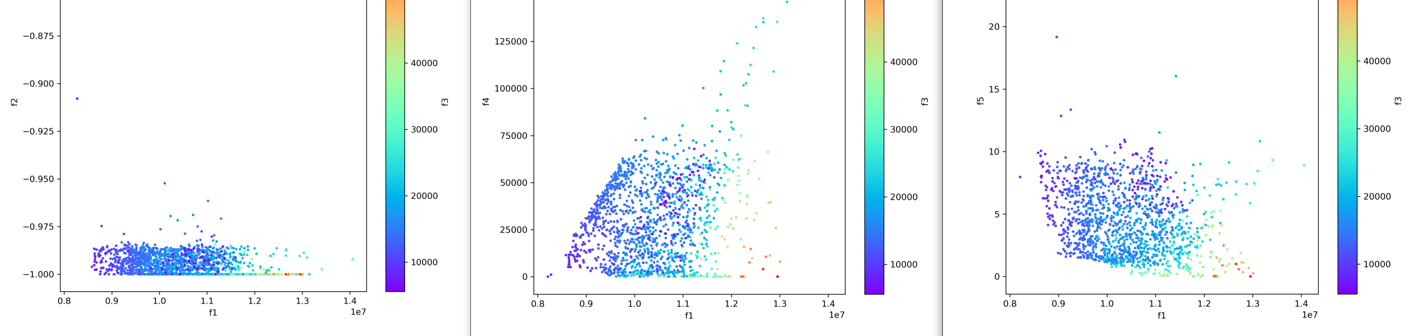
Since there are five objectives, each diagram shows three of them.
The Mazda Benchmark Problem
There are not many complex real-world multi-objective benchmark problems in the public domain. One of them is the Mazda Benchmark Problem, developed jointly by Mazda Motor Corporation, the Japan Aerospace Exploration Agency, and Tokyo University of Science. It has 222 discrete decision variables, 54 inequality constraints, and multiple objectives. The task is to design three cars at the same time while minimizing weight and maximizing the number of shared sheet-thickness parts, which reduces production cost. The original constraints represent expensive collision simulations used to assess car safety. In the benchmark, these simulations are replaced by response-surface approximations, which act as a domain-specific surrogate model. After generating solutions on the approximate model, the real collision simulations can be applied later to filter out solutions that do not hold up in the real world.
In Surrogate we described how to solve this problem with MODE, the fcmaes multi-objective algorithm.
With QD, the Mazda benchmark now yields more than 7000 diverse solutions, far more than a typical MO algorithm returns.
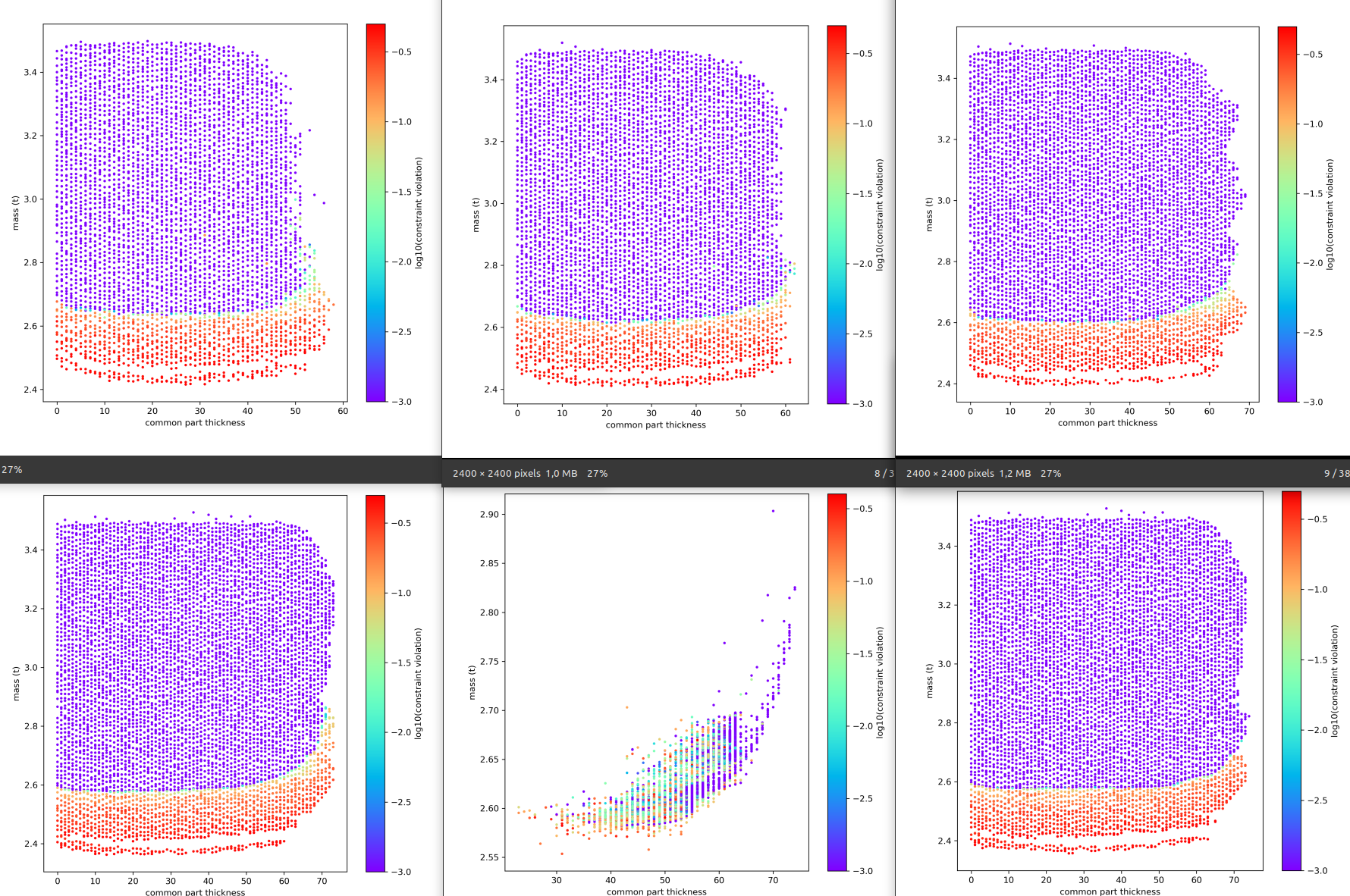
The figure above shows progress over time:
-
30 minutes: Hypervolume = 0.326 (only valid solutions)
-
1 hour: Hypervolume = 0.379
-
3 hours: Hypervolume = 0.428
-
10 hours: Hypervolume = 0.470
-
MO results: Hypervolume = 0.4959
-
merge with MO-results: Hypervolume = 0.498
The constraints approximate expensive physical simulations, namely crash tests. Satisfying the approximate constraints does not guarantee that the real constraints are also satisfied. The opposite can also happen: the approximation may be more restrictive than reality.
So not all 7000 solutions will be equally interesting. The most valuable ones may be the few hundred solutions near the border between valid and invalid regions. These can be the starting point for more detailed follow-up studies with more expensive simulations that verify the constraints.
QD defers the application of constraints
Constraints are still part of the QD optimization, but they are not enforced as strictly as in the MODE MO algorithm. Invalid solutions are kept in the archive together with valid ones. We can apply the final validity filter after the simulation. When the constraints are only approximations, that can be an advantage.
There are other reasons to defer the final application of constraints. The underlying assumptions may change. Suppose we want to know whether it is worth using a more expensive steel that relaxes some of the limits. Then we can derive the corresponding Pareto front from the optimization result we already have. The blue area would extend slightly further downward. That would show how many more common parts we could use in production, and we could compare the resulting cost savings with the higher material cost.
In terms of how many choices we have after optimization, the relation is simple: QD > MO > single objective. MO postpones the choice between objectives. QD does the same and also keeps invalid solutions for later inspection.
In 2017, Japan hosted a competition on this problem: Evolutionary Competition 2017. The goal was to reduce the gap between research in evolutionary computation and industry expectations. The multi-objective part of the competition produced this result:
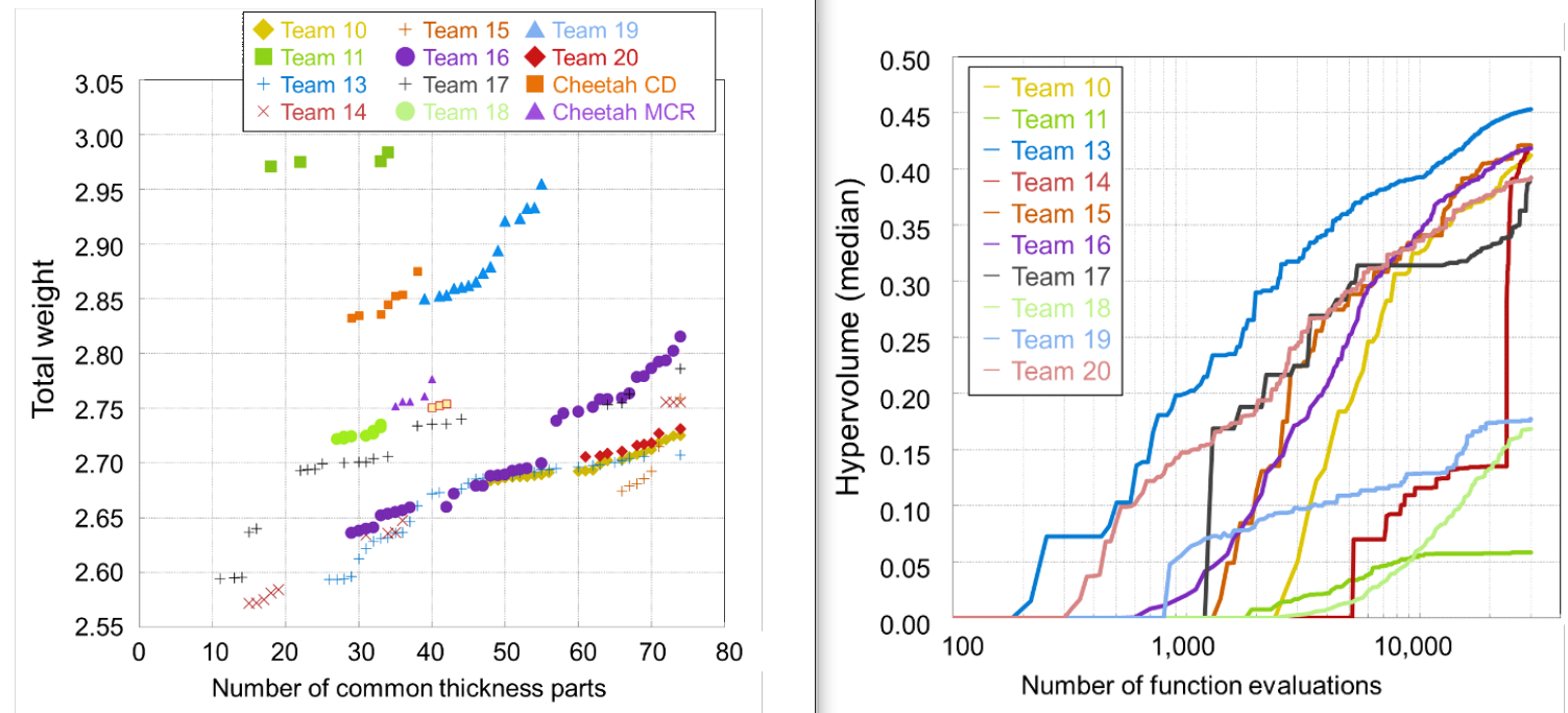
The figure shows only the best run out of 21, but the result achieved with only 30000 evaluations is still remarkable. Note that the winning team, team 13, used a single-objective algorithm called CR-FM-NES together with Tchebycheff scalarization of the constraints. That is why CR-FM-NES is now part of the fcmaes library and also part of Google’s EvoJax.
For QD, we use a weighted sum of the two objectives as the fitness value. The behavior vector contains the two objectives, and we add a penalty for constraint violations.
    class madzda_problem(object):

       def qd_fun(self, x):
           y = fitness(x)
           c = sum((y[self.nobj:] > 0)) # number of constraint violations
           b = y[:2].copy()
           constr = np.maximum(y[self.nobj:], 0)
           c += np.amax(constr) # maximum constraint violation
           y = (y[:2] - self.qd_bounds.lb) / (self.qd_bounds.ub - self.qd_bounds.lb)
           ws = sum(y[:nobj]) + c
           return ws, b

...
    problem.qd_dim = 2
    problem.qd_bounds = Bounds([2., -74], [3.5, 0])
    opt_params0 = {'solver':'elites', 'popsize':1000}
    opt_params1 = {'solver':'CRMFNES_CPP', 'max_evals':200000, 'popsize':32, 'stall_criterion':3}
    archive = diversifier.minimize(
         mapelites.wrapper(problem.qd_fun, 2, interval=100000, save_interval=2000000),
         problem.bounds, problem.qd_bounds, opt_params=[opt_params0, opt_params1], max_evals=400000000)
    print('final archive:', archive.info())
    archive.save('lrgv_qd')
We use CR-FM-NES as the base algorithm for the improvement emitter. In addition, CVT MAP-Elites uses half of the available threads. Both operate on the same multi-threaded QD archive. The QD fitness function qd_fun applies Tchebycheff scalarization to the constraints and returns the two objectives as the behavior vector.
Note that the original benchmark code was slightly modified to be thread-safe and directly accessible from Python. Parallelization is essential here. On an AMD 5950 16-core CPU, we can perform around 8000 simulations per second with 32 parallel threads.
Zooming into the QD-archive
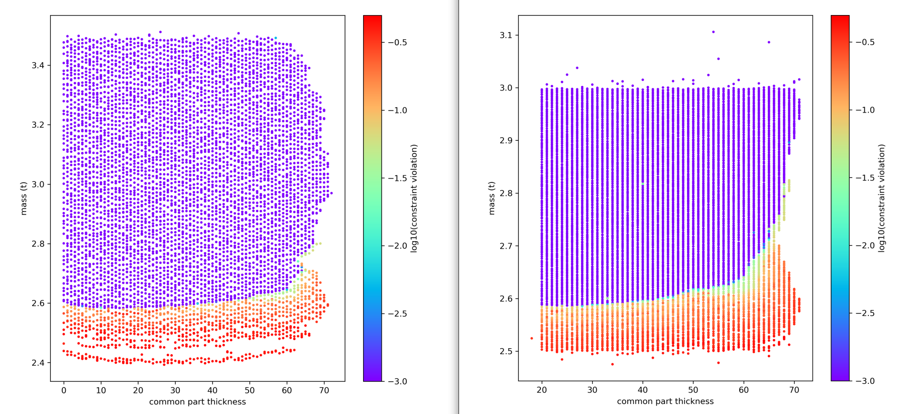
On the left, we see the QD result after 200 million fitness evaluations, which takes about 8 hours on a 16-core CPU. It was computed as follows:
niche_num = 10000

def nd_optimize():
    problem = madzda_problem()
    problem.qd_bounds = Bounds([2., -74], [3.5, 0])

    opt_params0 = {'solver':'elites', 'popsize':128}
    opt_params1 = {'solver':'CRMFNES_CPP', 'max_evals':200000, 'popsize':32, 'stall_criterion':3}
    archive = diversifier.minimize(
         mapelites.wrapper(problem.qd_fun, 2, problem.bounds, problem.qd_bounds,
         opt_params=[opt_params0, opt_params1], max_evals=200000000, niche_num = niche_num)
    archive.save("mazda1")
We used 100x100 niches and qd_bounds = Bounds([2., -74], [3.5, 0]). Suppose we now want to zoom in on a sub-area of the QD space. We can load the archive, change the bounds and number of niches, recompute the fitness and behavior vectors, and continue the optimization:
    niche_num = 160*160

    problem = madzda_problem()
    problem.qd_bounds = Bounds([2.5, -74], [3.0, -20]) # new qd bounds
    # load old archive using old niche number
    arch = mapelites.load_archive('mazda1', problem.bounds, problem.qd_bounds, 10000)
    # extract solutions
    xs = arch.get_xs()
    # change archive capacity / number of niches
    arch.capacity = niche_num
    # reset archive / delete all existing solutions
    arch.reset()
    # change number samples per niche to avoid memory overflow
    arch.init_niches(samples_per_niche = 12)
    # recompute solutions - works even with changed QD-fitness
    mapelites.update_archive(arch, xs, problem.qd_fun)
    # continue QD-optimization
    archive = diversifier.minimize(...,archive=arch,...)
    archive.save("mazda2")
The result after a few more hours is shown in the diagram on the right. We greatly increase the number of good valid solutions for each value of shared part thickness. The larger number of niches slows down the optimization, though. Throughput drops from about 8000 to about 4500 fitness evaluations per second.
Applying a MO-algorithm
Next, let us compare this with a MO algorithm:
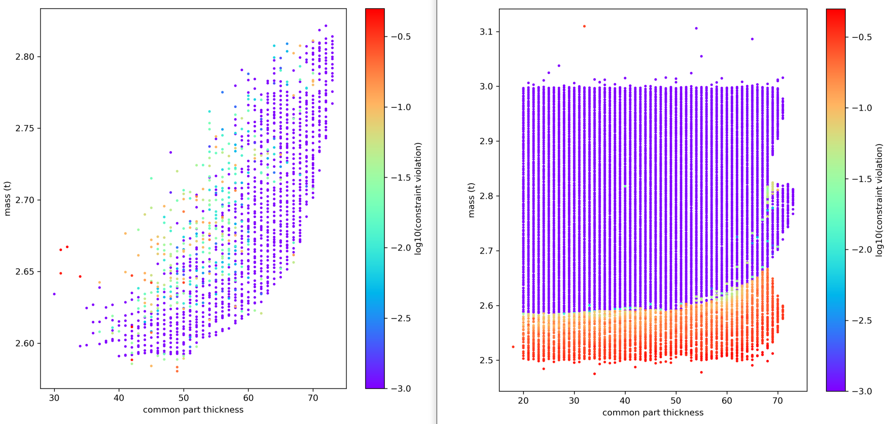
On the left, we see the result after the same number of fitness evaluations, 200 million. Computation time is slightly lower because there is no QD archive to maintain, so throughput rises to about 8800 evaluations per second.
    fun = mode.wrapper(problem.fun, problem.nobj, store, plot=False)
    x, y = modecpp.retry(fun,
                         problem.nobj, problem.ncon, problem.bounds, popsize = 256,
                         num_retries = 32, max_evaluations = 6250000, ints = np.array([True]*dim),
                         nsga_update=False)
    np.savez_compressed('mo_result', xs=x, ys=y)
We run 32 optimizations in parallel using the DE population update (nsga_update=False) and mark all decision variables as discrete (ints = np.array([True]*dim)). Finally, we use numpy’s savez_compressed to store all results, not just the Pareto front.
Hypervolume is better than with QD, but we get fewer alternatives to choose from. The MO fitness function problem.fun returns the two objectives and the 54 constraints separately. We do not need to weight them, because the MO algorithm handles them directly.
Still, MO algorithms should not be seen as competition here. They are a complement.
Join MO-algorithm results
We can simply merge the MO result into the QD archive and continue the QD optimization:
with np.load('mo_result') as data:
    xs2 =  np.array(data['xs']))
    arch = mapelites.load_archive('mazda2', problem.bounds, problem.qd_bounds, niche_num)
    # extract solutions
    xs = arch.get_xs()
    # reset archive / delete all existing solutions
    arch.reset()
    # recompute solutions - works even with changed QD-fitness
    mapelites.update_archive(arch, list(xs) + list(xs2), problem.qd_fun)
    # continue QD-optimization
    archive = diversifier.minimize(...,archive=arch,...)
    archive.save("mazda3")
The final result is shown on the right side of the figure above. If two machines are available, QD and MO optimization can also be run in parallel to save time.
Conclusion
There is still little literature on applying QD methods to expensive simulations, so there is not much we can compare against. These results are therefore preliminary, but they can still serve as a useful baseline for future work.
We found that:
-
CR-FM-NES can beat CMA-ES on many problems when used as an improvement emitter.
-
Mixing MAP-Elites with a CR-FM-NES improvement emitter works very well in most cases and should usually be the first configuration to try.
-
Sharing one QD archive between many parallel MAP-Elites and improvement-emitter processes often scales better than parallelizing the simulation itself.
-
fcmaes disables BLAS-level parallelism to avoid creating too many threads. The simulation itself should run single-threaded.
-
The default fcmaes configuration works well, but the population size can be adapted to the number of fitness evaluations your budget allows. A larger population size also reduces tessellation overhead by increasing the batch size. Compared with MO algorithms, population size is less critical here.
-
MAP-Elites can be configured to use Iso+LineDD, but for the problems tested here the default SBX plus mutation borrowed from NSGA-II works better. You can still try Iso+LineDD to improve an existing QD archive.
-
Improvement emitters are often initialized with niche elites. We found no problem where that worked better than random initialization, so we chose the latter.
-
MO algorithms are not competitors but complements to QD algorithms because they have different strengths and weaknesses. We can merge MO results into an existing QD archive.
-
fcmaes lets you change the number of niches, the fitness function, behavior limits, and other parameters before continuing the QD optimization. This makes it possible to drill down into interesting sub-areas of the behavior space.