fcmaes - a Python 3 gradient-free optimization library

Customized Surrogate Models

This tutorial

discusses customized surrogate models using the Mazda car design optimization problem
compares this approach with the use of a generic surrogate model.

Motivation

Since 2006 I have participated in the GTOC competition on global space trajectory optimization problems. Up to 2022 there were eleven competitions. Each one included problems that are hard to solve without a surrogate model that approximates the real-world model described in the task. In almost all cases, participants used a customized domain-specific surrogate. See Tutorials for details about the first competition Save the Earth. There, continuous thrust defined by ODEs is approximated by Lambert transfers. Local optimization is then applied to trajectory segments to turn the surrogate solution into one that satisfies the ODEs of the real problem.

The same idea also appears outside space flight dynamics.

Another example is the Mazda Benchmark Problem, jointly developed by the Mazda Motor Corporation, Japan Aerospace Exploration Agency, and Tokyo University of Science. It is a multi-objective problem with 222 discrete decision variables and 54 inequality constraints. Three cars are designed at the same time. The goals are to minimize their combined weight and maximize the number of common thickness parts across the three car types, because that reduces production cost. The original constraints use collision simulations to evaluate safety. In the benchmark, these expensive simulations are replaced by response surface approximations. These approximations already act as a domain-specific surrogate model. After generating solutions for the approximated model, real collision simulations can be used to filter solutions that also remain valid in the real world.

Should we add another "generic surrogate layer" on top of this problem? To answer that question, we compare with results from Large Scale Discrete Constrained Black Box Optimization Using Radial Basis Functions. The paper contains an interesting and debatable statement:

"However, when one single objective or constraint function evaluation potentially takes many hours, which is the case for many practical problems, this computational overhead is relatively small, and it makes sense to use a surrogate-based method given the substantial improvement in the best feasible solution obtained through the surrogate."

"Surrogate" in this statement means generic surrogate methods such as radial basis functions. Here the point is simpler:

It is a bad idea to apply a generic surrogate model to a problem that already has a domain-specific surrogate model and therefore allows a large number of function / constraint evaluations.

A result that needs about 6 hours with the method from the paper needs about 8 seconds with fcmaes. We use a cheap 600$ CPU (AMD5950x), so the difference is not caused by unusual hardware. Parallel function evaluation enables about 6000 evaluations per second, including the 54 constraints and the optimization overhead. In the paper, only 4000 function evaluations are required. But that does not help if those evaluations take more than 6 hours instead of about a second. In addition, our optimization starts from a random population and does not require a feasible input solution, unlike CONDOR, the method from the paper.

That leads to the broader question:

Should we apply a generic or a domain-specific customized surrogate model? A generic surrogate is often easier to apply, but in many domains, such as space flight dynamics and car design, reusable domain-specific surrogate models already exist.

Even when a domain-specific surrogate is not available, there are other ways to speed up the simulation:

Parallelization: Utilizing all cores of the CPU.
Clusterization: Distributing expensive simulations across separate cluster nodes. See Temporal-tutorial for an example.
Applying numba can speed up simulations by a factor of 10-100, as shown in Crypto Trading, Noisy TSP, JobShop and Scheduling.

Most generic surrogate methods, with the exception of MVRSM, share one weakness:

They are very good for the first few hundred function evaluations, but often do not scale well to larger budgets.

Car design

From the README, section "Engineering Design Optimization", we already know that the MODE algorithm can solve the two-objective Mazda car design task. This problem requires a corresponding shared library, which is not included in fcmaes for licensing reasons. We therefore show how to define the objective function, but the code cannot be executed without that shared library.

Single objective variant results

To compare with Large Scale Discrete Constrained Black Box Optimization Using Radial Basis Functions. we use a single-objective variant of the Mazda car design problem that optimizes only the combined masses of the car models. In practice, this variant is of limited value, because too few shared part thicknesses tend to increase production cost. It is also an order of magnitude easier to solve than the two-objective variant, as we will see later. A good feasible solution appears after only a few seconds. One option is Differential Evolution with a weighted-sum approach for the constraints:

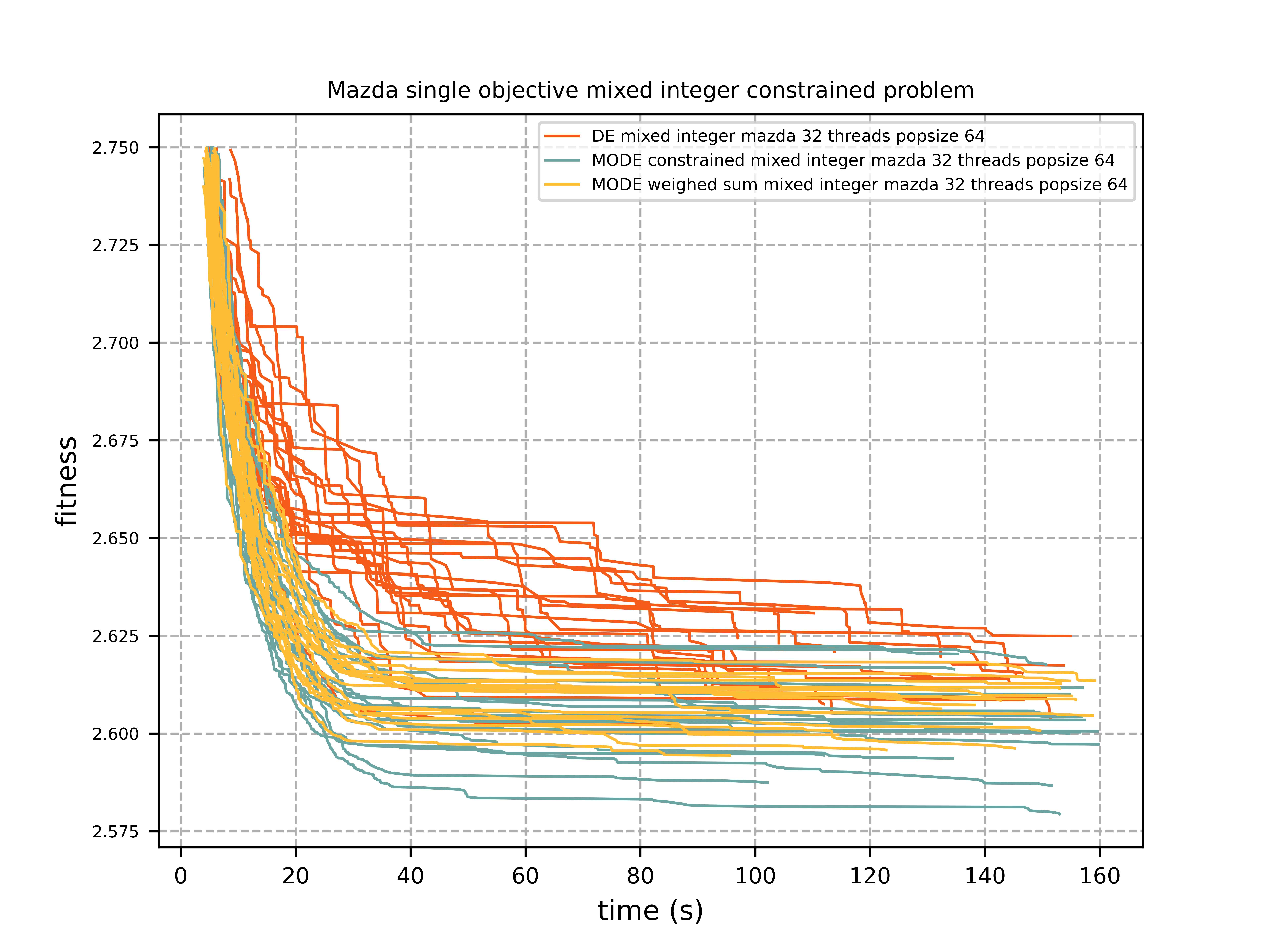
The following image compares three methods with a time budget of 160 seconds on an AMD 5950x using 32 threads:

fcmaes Differential Evolution, population size = 64, weighted sum approach.
fcmaes MODE, nsga_update=False, population size = 64, using constraints.
fcmaes MODE, nsga_update=False, population size = 64, weighted sum approach.

The results show:

All fcmaes methods surpass the best result from Large Scale Discrete Constrained Black Box Optimization Using Radial Basis Functions (2.65) after a few seconds.
After 160 seconds, results between 2.578 and 2.625 are reached. Either more than 6 hours was still not enough, or initializing CONDOR with feasible solutions, while fcmaes starts from random solutions, traps the search in local minima.
fcmaes MODE works better here than fcmaes DE, even with a single objective and with the same weighted-sum approach for the constraints. One possible reason is the DE/rand/1 strategy (nsga_update=False); DE uses the DE/best/1 strategy.
fcmaes MODE works best with explicit constraints, since these are prioritized by the algorithm.

Note that both DE and MODE use the ints = np.array([True]*dim) parameter to indicate that all decision variables are discrete.

Mazda single objective mixed integer constrained problem

Multi objective variant results

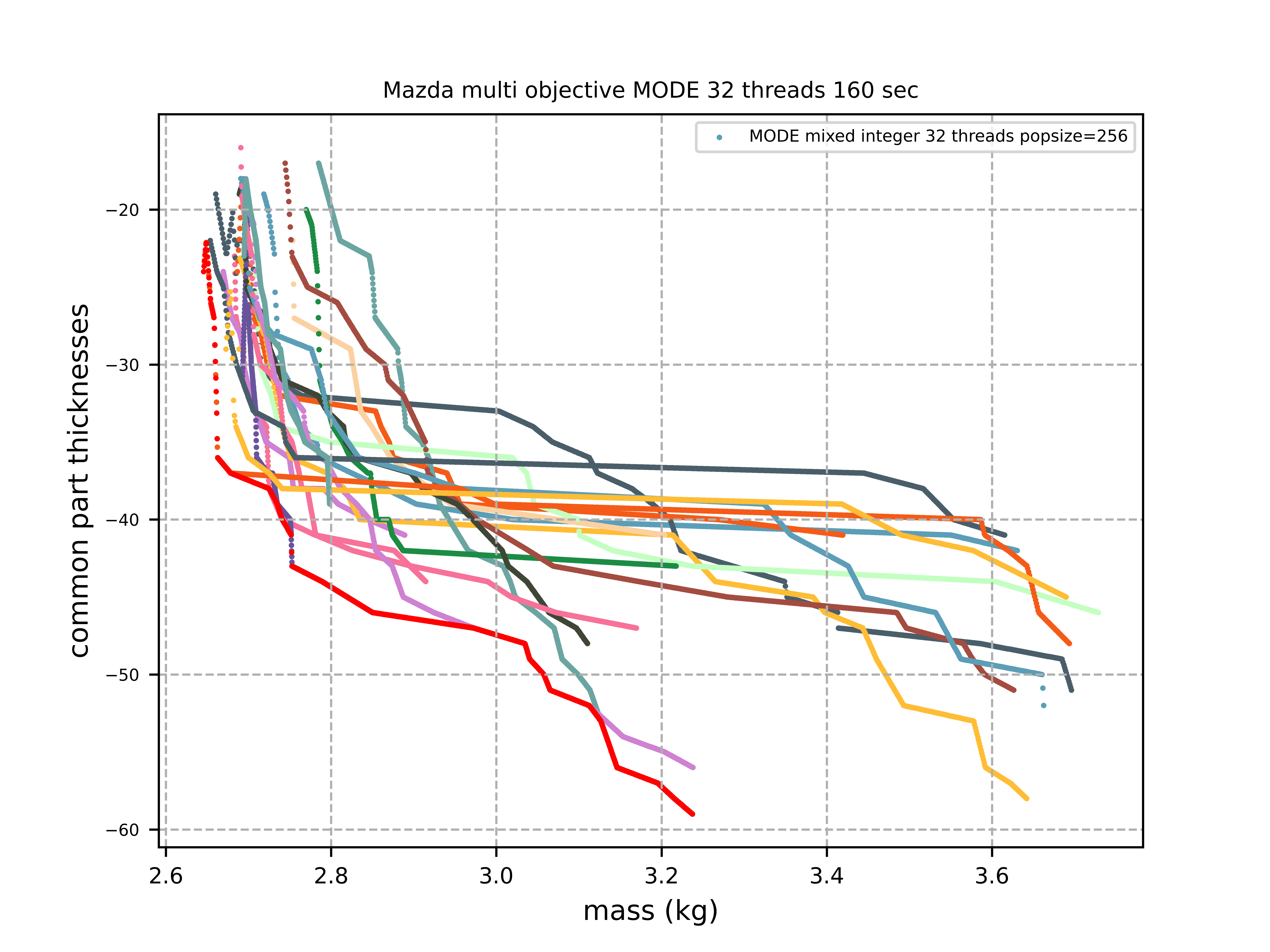
The multi-objective variant optimizes both the car masses and the number of shared part thicknesses. The first figure shows all Pareto fronts computed after 160 seconds on an AMD 5950x CPU using 32 threads, across about 20 optimization runs. Best masses vary between 2.65 and 2.79, and the best numbers of common part thicknesses vary between 41 and 59. The red line is the Pareto front obtained by combining all 20 runs.

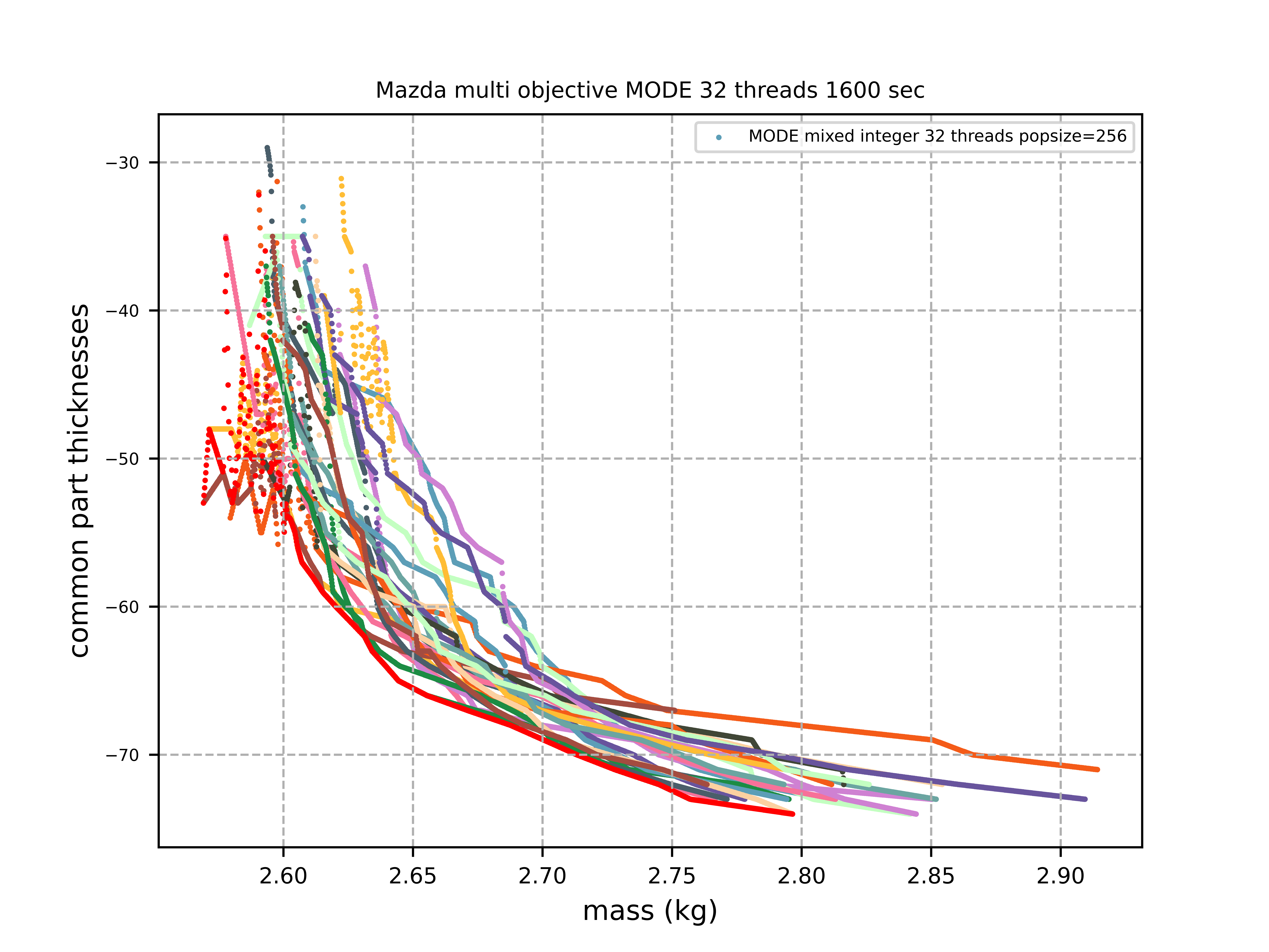
Mazda multi objective MODE 32 threads 160 sec

Increasing the time budget by a factor of 10 to 1600 sec changes the picture significantly. Best masses vary between 2.57 and 2.63, and the best numbers of common part thicknesses vary between 71 and 74. Even for a good mass of 2.7, we get 64 - 69 common parts. The 20 runs are quite consistent. The red line, which combines all runs, can serve as a reference for other methods and points to a significant reduction in production cost. We could not reproduce these results with NSGA-II update (nsga_update=True), although that setting proved superior for other problems.

Mazda multi objective MODE 32 threads 1600 sec

The picture above suggests another idea. Instead of parallel function evaluation, we can use parallel retries and take the combined Pareto front as the result:

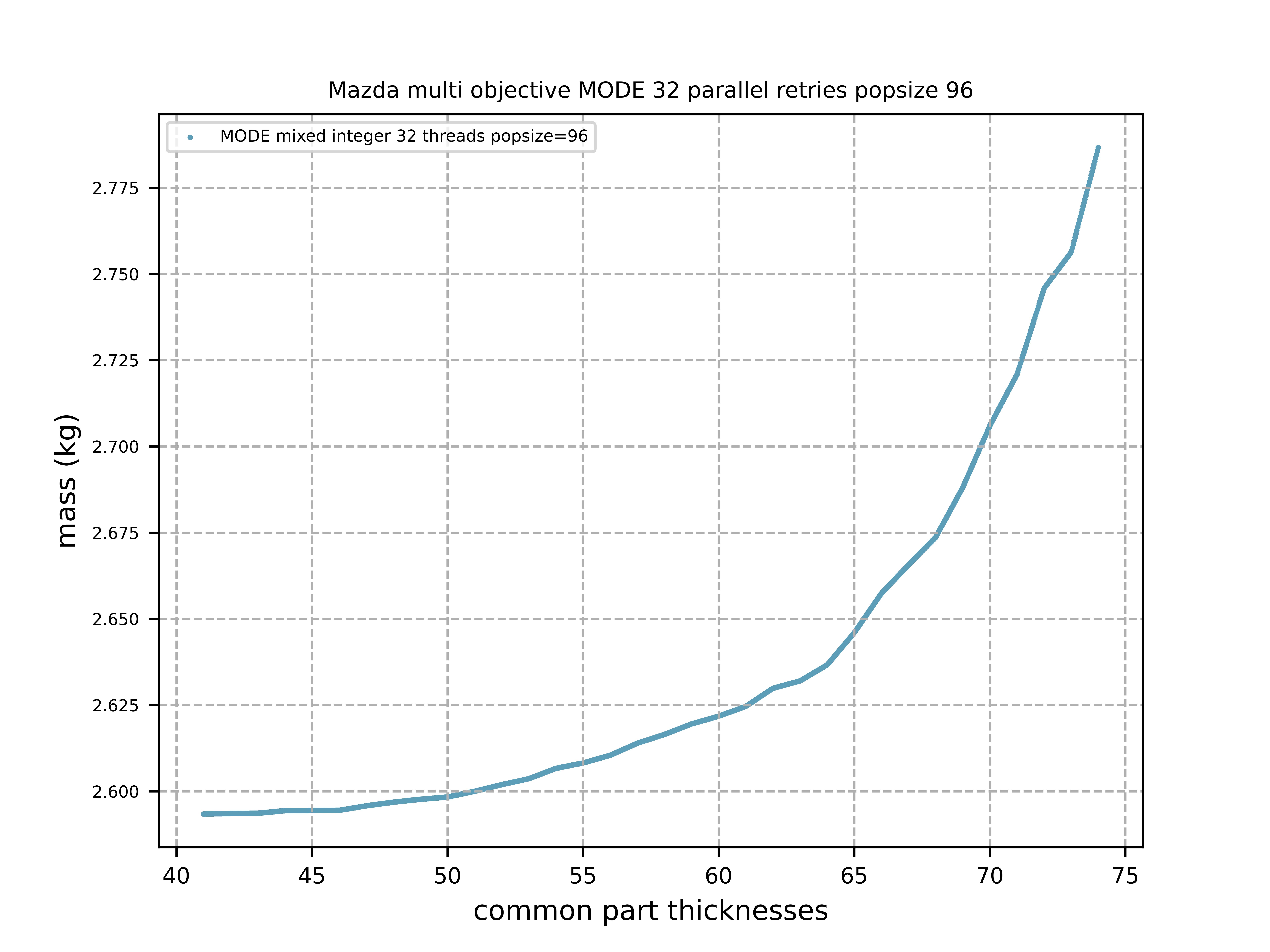
Mazda multi objective MODE 32 parallel retries popsize 96

We exchanged the x- and y-axis to enable direct comparison with the Evolutionary Competition 2017 results:

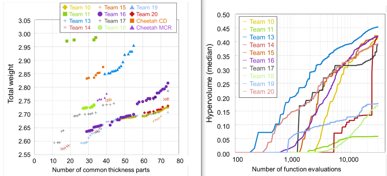
In the competition, there was an evaluation limit of 30000. Under that limit, the shown results are excellent. Unfortunately, the algorithms do not seem to be available as open source, so they are hard to reproduce. A hypervolume of 0.45 after 30000 evaluations is very fast. MODE converges much more slowly:

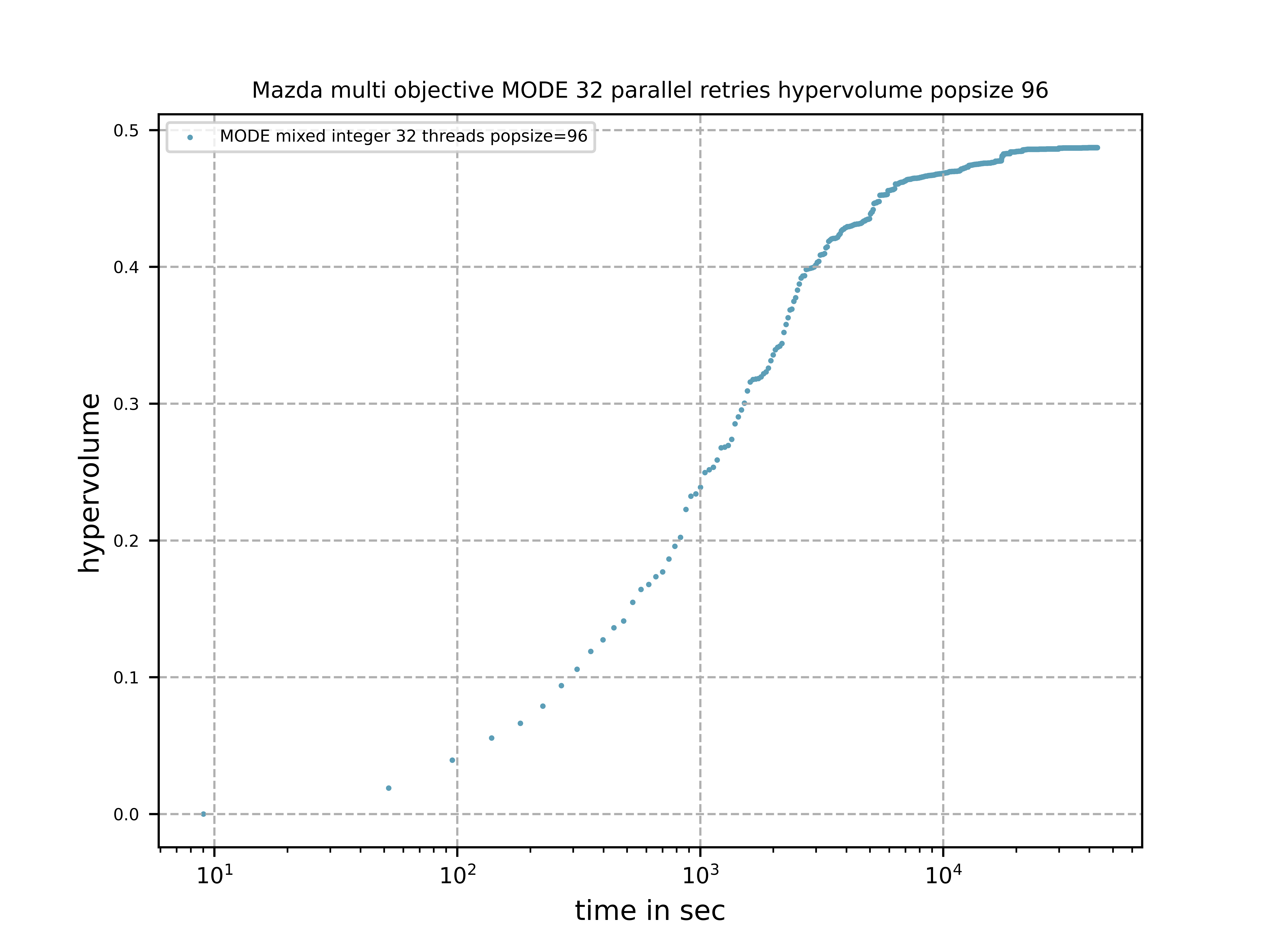
Mazda multi objective MODE 32 parallel retries hypervolume popsize 96

On the other hand, if you really want to produce the three car models at a combined mass of 2.625, the best competition results show 31 common part thicknesses. MODE reaches 62, about twice as many, although the hypervolume looks similar: 0.49 for MODE and 0.45 for the best competition results. The difference between 62 and 31 common part thicknesses has a significant impact on production cost. That means the competition results are not very relevant in practice. Whether 10 hours of execution time on a single mainstream CPU is really an issue depends on the use case. Unfortunately, we cannot check whether, or with which evaluation and time budget, the competition methods can reach hypervolume 0.49.

Reference Solution

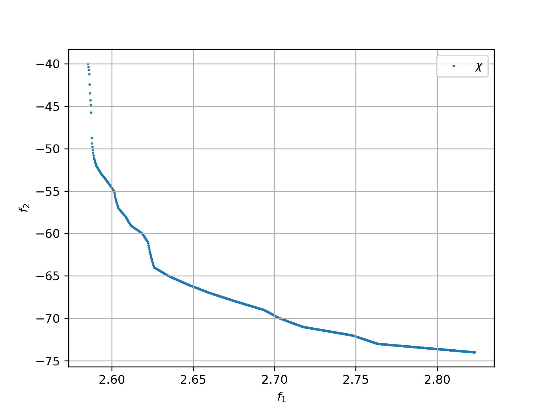
The following optimizer configuration was used to produce the Hypervolume = 0.4959 reference solution shown below.

            x, y = modecpp.retry(fun, problem.nobj, problem.ncon, problem.bounds, popsize = 256,
                                max_evaluations = 5000000, ints = np.array([True]*dim),
                                nsga_update=False, num_retries = 16, workers=16)
            np.savez_compressed(pname, xs=x, ys=y)
            moretry.plot(pname, problem.ncon, x, y)

16 parallel mode optimization runs were executed, and their Pareto fronts were joined, with 5E6 evaluations each. This setup was executed twice in parallel on the AMD 5950x 16 core CPU to maximize CPU utilization. The combined evaluation rate was 8400 evals/second.

Wrapping the objective function

First download the Mazda sources. We show everything only for the three-car problem. The two-car problem is very similar.

Calling the C++ code through the command line adds significant overhead, much more than the function execution itself. There are also only executables for linux+win64. We therefore enable direct calls from Python and add the following to mazda_mop.cpp:

extern "C" {

    void fitness_MazdaMop_C(double* x, int dim, double* objs, double* constr) {
        try {
            bp::MazdaMop mop;
            if (dim != mop.nvar) {
                cerr << "[Error] The number of variables is different from the benchmark problem." << endl;
                cerr << "dim: " << dim << endl;
                cerr << "benchmark problem: " << mop.nvar << endl;
                return;
            }
            vector<double> var(mop.nvar);
            for (int i = 0; i < mop.nvar; i++)
                var[i] = x[i];
            vector<double> obj(mop.nobj);
            vector<double> con(mop.ncon);
            mop.evaluate(var, obj, con);
            for (int i = 0; i < mop.nobj; i++)
                objs[i] = obj[i];
            for (int i = 0; i < mop.ncon; i++)
                constr[i] = con[i];
            var.clear();
            obj.clear();
            con.clear();
        } catch (std::exception &e) {
            cout << e.what() << endl;
        }
    }
}

Undefine the cout << "[Info] Acknowledge of your … line, because it does not work when called from Python.

Next we create a CMakeList.txt to build the library file.

set(CMAKE_CXX_FLAGS "${CMAKE_CXX_FLAGS} -std=gnu++11")
set(CMAKE_CXX_FLAGS_RELEASE "-O3 -DNDEBUG -march=native")
INCLUDE_DIRECTORIES(/path_to/Mazda_CdMOBP/Mazda_CdMOBP/src/RSM/)

if(NOT CMAKE_BUILD_TYPE)
   set(CMAKE_BUILD_TYPE "Release" CACHE STRING
      "Choose the type of build, options are: Debug Release
      RelWithDebInfo MinSizeRel." FORCE)
endif()

PROJECT(mazda)
add_library(mazda SHARED mazda_mop.cpp mazda_mop_sca.cpp RSM/g01_SUV_FrFL.cpp  RSM/g20_LV_ODB.cpp RSM/g39_SV_ODB.cpp RSM/g02_SUV_ODB.cpp   RSM/g21_LV_ODB.cpp   RSM/g40_SV_ODB.cpp RSM/g03_SUV_ODB.cpp   RSM/g22_LV_ODB.cpp   RSM/g41_SV_SIDE.cpp RSM/g04_SUV_ODB.cpp   RSM/g23_LV_SIDE.cpp  RSM/g42_SV_SIDE.cpp RSM/g05_SUV_SIDE.cpp  RSM/g24_LV_SIDE.cpp  RSM/g43_SV_SIDE.cpp RSM/g06_SUV_SIDE.cpp  RSM/g25_LV_SIDE.cpp  RSM/g44_SV_REAR.cpp RSM/g07_SUV_SIDE.cpp  RSM/g26_LV_REAR.cpp  RSM/g45_SV_REAR.cpp RSM/g08_SUV_REAR.cpp  RSM/g27_LV_REAR.cpp  RSM/g46_SV_LEV.cpp RSM/g09_SUV_REAR.cpp  RSM/g28_LV_LEV.cpp   RSM/g47_SV_LEV.cpp RSM/g10_SUV_LEV.cpp   RSM/g29_LV_LEV.cpp   RSM/g48_SV_LEV.cpp RSM/g11_SUV_LEV.cpp   RSM/g30_LV_LEV.cpp   RSM/g49_SV_BS.cpp RSM/g12_SUV_LEV.cpp   RSM/g31_LV_BS.cpp    RSM/g50_SV_BS.cpp RSM/g13_SUV_BS.cpp    RSM/g32_LV_BS.cpp    RSM/m01_SUV_Mass.cpp RSM/g14_SUV_BS.cpp    RSM/g37_SV_FrFL.cpp  RSM/m02_LV_Mass.cpp RSM/g19_LV_FrFL.cpp   RSM/g38_SV_ODB.cpp   RSM/m03_SV_Mass.cpp )

set(CMAKE_INSTALL_LIBDIR ${CMAKE_BINARY_DIR}/../Mazda_CdMOBP/lib)

After running cmake and make, we should get a libmazda.so / libmazda.dll file that Python can load:

We can then load the library from Python:

basepath = os.path.dirname(os.path.abspath(__file__))
if sys.platform.startswith('linux'):
    libmazda = ct.cdll.LoadLibrary(basepath + '/../fcmaes/lib/libmazda.so')
else:
    os.environ['PATH'] = (basepath + '/lib') + os.pathsep + os.environ['PATH']
    libmazda = ct.cdll.LoadLibrary(basepath + '/../fcmaes/lib/libmazda.dll')

fitness_MazdaMop = libmazda.fitness_MazdaMop_C
fitness_MazdaMop.argtypes = [ct.POINTER(ct.c_double), ct.c_int, ct.POINTER(ct.c_double), ct.POINTER(ct.c_double)]

From Info_Mazda_CdMOBP.xlsx, we need to copy the discrete values for the 222 decision variables and define fitness(x), which calls the C++ library:

dim = 222
nobj = 5
ncon = 54
decision_x = [   \
    [0.9, 0.95, 1.0, 1.2, 1.4, 1.5], \
    [0.3, 0.35, 0.4, 0.45, 0.5, 0.55, 0.6, 0.65, 0.7, 0.75, 0.8, 0.85, 0.9, 0.95], \
    [1.1, 1.2, 1.4, 1.6, 1.8, 2.0, 2.1], \
    [0.35, 0.4, 0.45, 0.5, 0.55, 0.6, 0.65, 0.7, 0.75, 0.8, 0.85, 0.9, 0.95, 1.0], \
    [1.5, 1.6, 1.8, 2.0, 2.2, 2.3], \
    [0.5, 0.55, 0.6, 0.65, 0.7, 0.75, 0.8, 0.85, 0.9, 0.95, 1.0, 1.2, 1.4, 1.6, 1.8, 2.0, 2.1], \
    [1.3, 1.4, 1.6, 1.8, 2.0, 2.1], \
    [1.7, 1.8, 2.0, 2.2, 2.3], \
    [1.1, 1.2, 1.4, 1.6, 1.7], \
    [0.7, 0.75, 0.8, 0.85, 0.9, 0.95, 1.0, 1.2, 1.4, 1.5], \
    [1.7, 1.8, 2.0, 2.2, 2.3, 2.4, 2.6], \
    [0.5, 0.55, 0.6, 0.65, 0.7, 0.75, 0.8, 0.85, 0.9, 0.95, 1.0, 1.2, 1.3], \
    [1.1, 1.2, 1.4, 1.6, 1.7], \
    [1.3, 1.4, 1.6, 1.8, 1.9], \
    [1.1, 1.2, 1.4, 1.6, 1.7], \
    [1.3, 1.4, 1.6, 1.8, 1.9], \
    [0.9, 0.95, 1.0, 1.2, 1.4, 1.6, 1.8, 2.0, 2.1], \
    [1.1, 1.2, 1.4, 1.6, 1.8, 1.9], \
    [1.5, 1.6, 1.8, 2.0, 2.2, 2.3], \
    [0.9, 0.95, 1.0, 1.2, 1.4, 1.5], \
    [0.9, 0.95, 1.0, 1.2, 1.4, 1.5], \
    [0.5, 0.55, 0.6, 0.65, 0.7, 0.75, 0.8, 0.85, 0.9, 0.95, 1.0, 1.1], \
    [0.5, 0.55, 0.6, 0.65, 0.7, 0.75, 0.8, 0.85, 0.9, 0.95, 1.0, 1.2], \
    [0.9, 0.95, 1.0, 1.2, 1.4, 1.6, 1.8, 2.0, 2.1], \
    [0.3, 0.35, 0.4, 0.45, 0.5, 0.55, 0.6, 0.65, 0.7, 0.75, 0.8, 0.85, 0.9], \
    [0.4, 0.45, 0.5, 0.55, 0.6, 0.65, 0.7, 0.75, 0.8, 0.85, 0.9, 0.95, 1.0], \
    [1.3, 1.4, 1.6, 1.8, 1.9], \
    [0.6, 0.65, 0.7, 0.75, 0.8, 0.85, 0.9, 0.95, 1.0, 1.2, 1.3], \
    [0.6, 0.65, 0.7, 0.75, 0.8, 0.85, 0.9, 0.95, 1.0, 1.2], \
    [0.4, 0.45, 0.5, 0.55, 0.6, 0.65, 0.7, 0.75, 0.8, 0.85, 0.9, 0.95, 1.0, 1.2, 1.4, 1.6, 1.7], \
    [0.9, 0.95, 1.0, 1.2, 1.4, 1.6, 1.8, 1.9], \
    [0.6, 0.65, 0.7, 0.75, 0.8, 0.85, 0.9, 0.95, 1.0, 1.2, 1.3], \
    [0.9, 0.95, 1.0, 1.2, 1.4, 1.6, 1.7], \
    [0.7, 0.75, 0.8, 0.85, 0.9, 0.95, 1.0, 1.2, 1.3], \
    [0.4, 0.45, 0.5, 0.55, 0.6, 0.65, 0.7, 0.75, 0.8, 0.85, 0.9, 0.95, 1.0, 1.2, 1.4, 1.6, 1.8, 1.9], \
    [1.5, 1.6, 1.8, 2.0, 2.2, 2.3], \
    [0.6, 0.65, 0.7, 0.75, 0.8, 0.85, 0.9, 0.95, 1.0, 1.2], \
    [0.3, 0.35, 0.4, 0.45, 0.5, 0.55, 0.6, 0.65, 0.7, 0.75, 0.8, 0.85, 0.9], \
    [0.3, 0.35, 0.4, 0.45, 0.5, 0.55, 0.6, 0.65, 0.7, 0.75, 0.8, 0.85, 0.9], \
    [0.6, 0.65, 0.7, 0.75, 0.8, 0.85, 0.9, 0.95, 1.0, 1.2], \
    [1.7, 1.8, 2.0, 2.2, 2.3], \
    [0.9, 0.95, 1.0, 1.2, 1.4, 1.6, 1.7], \
    [0.5, 0.55, 0.6, 0.65, 0.7, 0.75, 0.8, 0.85, 0.9, 0.95, 1.0, 1.1], \
    [1.3, 1.4, 1.6, 1.8, 1.9], \
    [0.7, 0.75, 0.8, 0.85, 0.9, 0.95, 1.0, 1.2, 1.4, 1.6, 1.7], \
    [0.7, 0.75, 0.8, 0.85, 0.9, 0.95, 1.0, 1.2, 1.4, 1.6, 1.8, 2.0, 2.1], \
    [0.9, 0.95, 1.0, 1.2, 1.4, 1.6, 1.8, 2.0, 2.1], \
    [1.3, 1.4, 1.6, 1.8, 2.0, 2.1], \
    [1.1, 1.2, 1.4, 1.6, 1.8, 1.9], \
    [1.3, 1.4, 1.6, 1.8, 2.0, 2.1], \
    [2.0, 2.2, 2.3, 2.4, 2.6], \
    [1.7, 1.8, 2.0, 2.2, 2.3], \
    [1.1, 1.2, 1.4, 1.6, 1.7], \
    [0.9, 0.95, 1.0, 1.2, 1.4, 1.6, 1.8, 2.0, 2.1], \
    [0.3, 0.35, 0.4, 0.45, 0.5, 0.55, 0.6, 0.65, 0.7, 0.75, 0.8, 0.85, 0.9], \
    [0.6, 0.65, 0.7, 0.75, 0.8, 0.85, 0.9, 0.95, 1.0, 1.2, 1.3], \
    [0.9, 0.95, 1.0, 1.2, 1.4, 1.6, 1.7], \
    [1.1, 1.2, 1.4, 1.6, 1.8, 1.9], \
    [1.3, 1.4, 1.6, 1.8, 1.9], \
    [0.3, 0.35, 0.4, 0.45, 0.5, 0.55, 0.6, 0.65, 0.7, 0.75, 0.8, 0.85, 0.9, 0.95, 1.0, 1.2, 1.3], \
    [0.3, 0.35, 0.4, 0.45, 0.5, 0.55, 0.6, 0.65, 0.7, 0.75, 0.8, 0.85, 0.9, 0.95, 1.0, 1.1], \
    [1.3, 1.4, 1.6, 1.8, 1.9], \
    [0.9, 0.95, 1.0, 1.2, 1.4, 1.5], \
    [1.1, 1.2, 1.4, 1.6, 1.7], \
    [0.7, 0.75, 0.8, 0.85, 0.9, 0.95, 1.0, 1.2, 1.4, 1.6, 1.8, 2.0], \
    [1.7, 1.8, 2.0, 2.2, 2.3], \
    [1.1, 1.2, 1.4, 1.6, 1.7], \
    [0.9, 0.95, 1.0, 1.2, 1.4, 1.6, 1.7], \
    [0.7, 0.75, 0.8, 0.85, 0.9, 0.95, 1.0, 1.2, 1.4, 1.6, 1.8, 2.0, 2.1], \
    [1.1, 1.2, 1.4, 1.6, 1.8, 1.9], \
    [0.9, 0.95, 1.0, 1.2, 1.4, 1.6, 1.7], \
    [1.7, 1.8, 2.0, 2.2, 2.3], \
    [2.0, 2.2, 2.3, 2.4, 2.6], \
    [0.5, 0.55, 0.6, 0.65, 0.7, 0.75, 0.8, 0.85, 0.9, 0.95, 1.0, 1.2, 1.3], \
    [0.9, 0.95, 1.0, 1.2, 1.4, 1.5], \
    [0.3, 0.35, 0.4, 0.45, 0.5, 0.55, 0.6, 0.65, 0.7, 0.75, 0.8, 0.85, 0.9, 0.95], \
    [1.1, 1.2, 1.4, 1.6, 1.8, 2.0, 2.1], \
    [0.35, 0.4, 0.45, 0.5, 0.55, 0.6, 0.65, 0.7, 0.75, 0.8, 0.85, 0.9, 0.95, 1.0], \
    [1.5, 1.6, 1.8, 2.0, 2.2, 2.3], \
    [0.5, 0.55, 0.6, 0.65, 0.7, 0.75, 0.8, 0.85, 0.9, 0.95, 1.0, 1.2, 1.4, 1.6, 1.8, 2.0, 2.1], \
    [1.3, 1.4, 1.6, 1.8, 2.0, 2.1], \
    [1.7, 1.8, 2.0, 2.2, 2.3], \
    [1.1, 1.2, 1.4, 1.6, 1.7], \
    [0.7, 0.75, 0.8, 0.85, 0.9, 0.95, 1.0, 1.2, 1.4, 1.5], \
    [1.7, 1.8, 2.0, 2.2, 2.3, 2.4, 2.6], \
    [0.5, 0.55, 0.6, 0.65, 0.7, 0.75, 0.8, 0.85, 0.9, 0.95, 1.0, 1.2, 1.3], \
    [1.1, 1.2, 1.4, 1.6, 1.7], \
    [1.3, 1.4, 1.6, 1.8, 1.9], \
    [1.1, 1.2, 1.4, 1.6, 1.7], \
    [1.3, 1.4, 1.6, 1.8, 1.9], \
    [0.9, 0.95, 1.0, 1.2, 1.4, 1.6, 1.8, 2.0, 2.1], \
    [1.1, 1.2, 1.4, 1.6, 1.8, 1.9], \
    [1.5, 1.6, 1.8, 2.0, 2.2, 2.3], \
    [0.9, 0.95, 1.0, 1.2, 1.4, 1.5], \
    [0.9, 0.95, 1.0, 1.2, 1.4, 1.5], \
    [0.5, 0.55, 0.6, 0.65, 0.7, 0.75, 0.8, 0.85, 0.9, 0.95, 1.0, 1.1], \
    [0.5, 0.55, 0.6, 0.65, 0.7, 0.75, 0.8, 0.85, 0.9, 0.95, 1.0, 1.2], \
    [0.9, 0.95, 1.0, 1.2, 1.4, 1.6, 1.8, 2.0, 2.1], \
    [0.3, 0.35, 0.4, 0.45, 0.5, 0.55, 0.6, 0.65, 0.7, 0.75, 0.8, 0.85, 0.9], \
    [0.4, 0.45, 0.5, 0.55, 0.6, 0.65, 0.7, 0.75, 0.8, 0.85, 0.9, 0.95, 1.0], \
    [1.3, 1.4, 1.6, 1.8, 1.9], \
    [0.6, 0.65, 0.7, 0.75, 0.8, 0.85, 0.9, 0.95, 1.0, 1.2, 1.3], \
    [0.6, 0.65, 0.7, 0.75, 0.8, 0.85, 0.9, 0.95, 1.0, 1.2], \
    [0.4, 0.45, 0.5, 0.55, 0.6, 0.65, 0.7, 0.75, 0.8, 0.85, 0.9, 0.95, 1.0, 1.2, 1.4, 1.6, 1.7], \
    [0.9, 0.95, 1.0, 1.2, 1.4, 1.6, 1.8, 1.9], \
    [0.6, 0.65, 0.7, 0.75, 0.8, 0.85, 0.9, 0.95, 1.0, 1.2, 1.3], \
    [0.9, 0.95, 1.0, 1.2, 1.4, 1.6, 1.7], \
    [0.7, 0.75, 0.8, 0.85, 0.9, 0.95, 1.0, 1.2, 1.3], \
    [0.4, 0.45, 0.5, 0.55, 0.6, 0.65, 0.7, 0.75, 0.8, 0.85, 0.9, 0.95, 1.0, 1.2, 1.4, 1.6, 1.8, 1.9], \
    [1.5, 1.6, 1.8, 2.0, 2.2, 2.3], \
    [0.6, 0.65, 0.7, 0.75, 0.8, 0.85, 0.9, 0.95, 1.0, 1.2], \
    [0.3, 0.35, 0.4, 0.45, 0.5, 0.55, 0.6, 0.65, 0.7, 0.75, 0.8, 0.85, 0.9], \
    [0.3, 0.35, 0.4, 0.45, 0.5, 0.55, 0.6, 0.65, 0.7, 0.75, 0.8, 0.85, 0.9], \
    [0.6, 0.65, 0.7, 0.75, 0.8, 0.85, 0.9, 0.95, 1.0, 1.2], \
    [1.7, 1.8, 2.0, 2.2, 2.3], \
    [0.9, 0.95, 1.0, 1.2, 1.4, 1.6, 1.7], \
    [0.5, 0.55, 0.6, 0.65, 0.7, 0.75, 0.8, 0.85, 0.9, 0.95, 1.0, 1.1], \
    [1.3, 1.4, 1.6, 1.8, 1.9], \
    [0.7, 0.75, 0.8, 0.85, 0.9, 0.95, 1.0, 1.2, 1.4, 1.6, 1.7], \
    [0.7, 0.75, 0.8, 0.85, 0.9, 0.95, 1.0, 1.2, 1.4, 1.6, 1.8, 2.0, 2.1], \
    [0.9, 0.95, 1.0, 1.2, 1.4, 1.6, 1.8, 2.0, 2.1], \
    [1.3, 1.4, 1.6, 1.8, 2.0, 2.1], \
    [1.1, 1.2, 1.4, 1.6, 1.8, 1.9], \
    [1.3, 1.4, 1.6, 1.8, 2.0, 2.1], \
    [2.0, 2.2, 2.3, 2.4, 2.6], \
    [1.7, 1.8, 2.0, 2.2, 2.3], \
    [1.1, 1.2, 1.4, 1.6, 1.7], \
    [0.9, 0.95, 1.0, 1.2, 1.4, 1.6, 1.8, 2.0, 2.1], \
    [0.3, 0.35, 0.4, 0.45, 0.5, 0.55, 0.6, 0.65, 0.7, 0.75, 0.8, 0.85, 0.9], \
    [0.6, 0.65, 0.7, 0.75, 0.8, 0.85, 0.9, 0.95, 1.0, 1.2, 1.3], \
    [0.9, 0.95, 1.0, 1.2, 1.4, 1.6, 1.7], \
    [1.1, 1.2, 1.4, 1.6, 1.8, 1.9], \
    [1.3, 1.4, 1.6, 1.8, 1.9], \
    [0.3, 0.35, 0.4, 0.45, 0.5, 0.55, 0.6, 0.65, 0.7, 0.75, 0.8, 0.85, 0.9, 0.95, 1.0, 1.2, 1.3], \
    [0.3, 0.35, 0.4, 0.45, 0.5, 0.55, 0.6, 0.65, 0.7, 0.75, 0.8, 0.85, 0.9, 0.95, 1.0, 1.1], \
    [1.3, 1.4, 1.6, 1.8, 1.9], \
    [0.9, 0.95, 1.0, 1.2, 1.4, 1.5], \
    [1.1, 1.2, 1.4, 1.6, 1.7], \
    [0.7, 0.75, 0.8, 0.85, 0.9, 0.95, 1.0, 1.2, 1.4, 1.6, 1.8, 2.0], \
    [1.7, 1.8, 2.0, 2.2, 2.3], \
    [1.1, 1.2, 1.4, 1.6, 1.7], \
    [0.9, 0.95, 1.0, 1.2, 1.4, 1.6, 1.7], \
    [0.7, 0.75, 0.8, 0.85, 0.9, 0.95, 1.0, 1.2, 1.4, 1.6, 1.8, 2.0, 2.1], \
    [1.1, 1.2, 1.4, 1.6, 1.8, 1.9], \
    [0.9, 0.95, 1.0, 1.2, 1.4, 1.6, 1.7], \
    [1.7, 1.8, 2.0, 2.2, 2.3], \
    [2.0, 2.2, 2.3, 2.4, 2.6], \
    [0.5, 0.55, 0.6, 0.65, 0.7, 0.75, 0.8, 0.85, 0.9, 0.95, 1.0, 1.2, 1.3], \
    [0.9, 0.95, 1.0, 1.2, 1.4, 1.5], \
    [0.3, 0.35, 0.4, 0.45, 0.5, 0.55, 0.6, 0.65, 0.7, 0.75, 0.8, 0.85, 0.9, 0.95], \
    [1.1, 1.2, 1.4, 1.6, 1.8, 2.0, 2.1], \
    [0.35, 0.4, 0.45, 0.5, 0.55, 0.6, 0.65, 0.7, 0.75, 0.8, 0.85, 0.9, 0.95, 1.0], \
    [1.5, 1.6, 1.8, 2.0, 2.2, 2.3], \
    [0.5, 0.55, 0.6, 0.65, 0.7, 0.75, 0.8, 0.85, 0.9, 0.95, 1.0, 1.2, 1.4, 1.6, 1.8, 2.0, 2.1], \
    [1.3, 1.4, 1.6, 1.8, 2.0, 2.1], \
    [1.7, 1.8, 2.0, 2.2, 2.3], \
    [1.1, 1.2, 1.4, 1.6, 1.7], \
    [0.7, 0.75, 0.8, 0.85, 0.9, 0.95, 1.0, 1.2, 1.4, 1.5], \
    [1.7, 1.8, 2.0, 2.2, 2.4, 2.6], \
    [0.5, 0.55, 0.6, 0.65, 0.7, 0.75, 0.8, 0.85, 0.9, 0.95, 1.0, 1.2, 1.3], \
    [1.1, 1.2, 1.4, 1.6, 1.7], \
    [1.3, 1.4, 1.6, 1.8, 1.9], \
    [1.1, 1.2, 1.4, 1.6, 1.7], \
    [1.3, 1.4, 1.6, 1.8, 1.9], \
    [0.9, 0.95, 1.0, 1.2, 1.4, 1.6, 1.8, 2.0, 2.1], \
    [1.1, 1.2, 1.4, 1.6, 1.8, 1.9], \
    [1.5, 1.6, 1.8, 2.0, 2.2, 2.3], \
    [0.9, 0.95, 1.0, 1.2, 1.4, 1.5], \
    [0.9, 0.95, 1.0, 1.2, 1.4, 1.5], \
    [0.5, 0.55, 0.6, 0.65, 0.7, 0.75, 0.8, 0.85, 0.9, 0.95, 1.0, 1.1], \
    [0.5, 0.55, 0.6, 0.65, 0.7, 0.75, 0.8, 0.85, 0.9, 0.95, 1.0, 1.2], \
    [0.9, 0.95, 1.0, 1.2, 1.4, 1.6, 1.8, 2.0, 2.1], \
    [0.3, 0.35, 0.4, 0.45, 0.5, 0.55, 0.6, 0.65, 0.7, 0.75, 0.8, 0.85, 0.9], \
    [0.4, 0.45, 0.5, 0.55, 0.6, 0.65, 0.7, 0.75, 0.8, 0.85, 0.9, 0.95, 1.0], \
    [1.3, 1.4, 1.6, 1.8, 1.9], \
    [0.6, 0.65, 0.7, 0.75, 0.8, 0.85, 0.9, 0.95, 1.0, 1.2, 1.3], \
    [0.6, 0.65, 0.7, 0.75, 0.8, 0.85, 0.9, 0.95, 1.0, 1.2], \
    [0.4, 0.45, 0.5, 0.55, 0.6, 0.65, 0.7, 0.75, 0.8, 0.85, 0.9, 0.95, 1.0, 1.2, 1.4, 1.6, 1.7], \
    [0.9, 0.95, 1.0, 1.2, 1.4, 1.6, 1.8, 1.9], \
    [0.6, 0.65, 0.7, 0.75, 0.8, 0.85, 0.9, 0.95, 1.0, 1.2, 1.3], \
    [0.9, 0.95, 1.0, 1.2, 1.4, 1.6, 1.7], \
    [0.7, 0.75, 0.8, 0.85, 0.9, 0.95, 1.0, 1.2, 1.3], \
    [0.4, 0.45, 0.5, 0.55, 0.6, 0.65, 0.7, 0.75, 0.8, 0.85, 0.9, 0.95, 1.0, 1.2, 1.4, 1.6, 1.8, 1.9], \
    [1.5, 1.6, 1.8, 2.0, 2.2, 2.3], \
    [0.6, 0.65, 0.7, 0.75, 0.8, 0.85, 0.9, 0.95, 1.0, 1.2], \
    [0.3, 0.35, 0.4, 0.45, 0.5, 0.55, 0.6, 0.65, 0.7, 0.75, 0.8, 0.85, 0.9], \
    [0.3, 0.35, 0.4, 0.45, 0.5, 0.55, 0.6, 0.65, 0.7, 0.75, 0.8, 0.85, 0.9], \
    [0.6, 0.65, 0.7, 0.75, 0.8, 0.85, 0.9, 0.95, 1.0, 1.2], \
    [1.7, 1.8, 2.0, 2.2, 2.3], \
    [0.9, 0.95, 1.0, 1.2, 1.4, 1.6, 1.7], \
    [0.5, 0.55, 0.6, 0.65, 0.7, 0.75, 0.8, 0.85, 0.9, 0.95, 1.0, 1.1], \
    [1.3, 1.4, 1.6, 1.8, 1.9], \
    [0.7, 0.75, 0.8, 0.85, 0.9, 0.95, 1.0, 1.2, 1.4, 1.6, 1.7], \
    [0.7, 0.75, 0.8, 0.85, 0.9, 0.95, 1.0, 1.2, 1.4, 1.6, 1.8, 2.0, 2.1], \
    [0.9, 0.95, 1.0, 1.2, 1.4, 1.6, 1.8, 2.0, 2.1], \
    [1.3, 1.4, 1.6, 1.8, 2.0, 2.1], \
    [1.1, 1.2, 1.4, 1.6, 1.8, 1.9], \
    [1.3, 1.4, 1.6, 1.8, 2.0, 2.1], \
    [2.0, 2.2, 2.3, 2.4, 2.6], \
    [1.7, 1.8, 2.0, 2.2, 2.3], \
    [1.1, 1.2, 1.4, 1.6, 1.7], \
    [0.9, 0.95, 1.0, 1.2, 1.4, 1.6, 1.8, 2.0, 2.1], \
    [0.3, 0.35, 0.4, 0.45, 0.5, 0.55, 0.6, 0.65, 0.7, 0.75, 0.8, 0.85, 0.9], \
    [0.6, 0.65, 0.7, 0.75, 0.8, 0.85, 0.9, 0.95, 1.0, 1.2, 1.3], \
    [0.9, 0.95, 1.0, 1.2, 1.4, 1.6, 1.7], \
    [1.1, 1.2, 1.4, 1.6, 1.8, 1.9], \
    [1.3, 1.4, 1.6, 1.8, 1.9], \
    [0.3, 0.35, 0.4, 0.45, 0.5, 0.55, 0.6, 0.65, 0.7, 0.75, 0.8, 0.85, 0.9, 0.95, 1.0, 1.2, 1.3], \
    [0.3, 0.35, 0.4, 0.45, 0.5, 0.55, 0.6, 0.65, 0.7, 0.75, 0.8, 0.85, 0.9, 0.95, 1.0, 1.1], \
    [1.3, 1.4, 1.6, 1.8, 1.9], \
    [0.9, 0.95, 1.0, 1.2, 1.4, 1.5], \
    [1.1, 1.2, 1.4, 1.6, 1.7], \
    [0.7, 0.75, 0.8, 0.85, 0.9, 0.95, 1.0, 1.2, 1.4, 1.6, 1.8, 2.0], \
    [1.7, 1.8, 2.0, 2.2, 2.3], \
    [1.1, 1.2, 1.4, 1.6, 1.7], \
    [0.9, 0.95, 1.0, 1.2, 1.4, 1.6, 1.7], \
    [0.7, 0.75, 0.8, 0.85, 0.9, 0.95, 1.0, 1.2, 1.4, 1.6, 1.8, 2.0, 2.1], \
    [1.1, 1.2, 1.4, 1.6, 1.8, 1.9], \
    [0.9, 0.95, 1.0, 1.2, 1.4, 1.6, 1.7], \
    [1.7, 1.8, 2.0, 2.2, 2.3], \
    [2.0, 2.2, 2.3, 2.4, 2.6], \
    [0.5, 0.55, 0.6, 0.65, 0.7, 0.75, 0.8, 0.85, 0.9, 0.95, 1.0, 1.2, 1.3], \
    ]

def fitness(x):
    try:
        x = np.array(x)
        y = np.empty(nobj)
        c = np.empty(ncon)
        x = np.array([decision_x[i][int(xi)] for i, xi in enumerate(x)])
        x_p = x.ctypes.data_as(ct.POINTER(ct.c_double))
        y_p = y.ctypes.data_as(ct.POINTER(ct.c_double))
        c_p = c.ctypes.data_as(ct.POINTER(ct.c_double))
        if two_cars:
            fitness_MazdaMop_sca(x_p, dim, y_p, c_p)
        else:
            fitness_MazdaMop(x_p, dim, y_p, c_p)
        return np.array(list(y[:2]) + list(c * -1))
    except Exception as ex:
        return None

We are interested only in the first two objectives, and we need to negate the constraint values. That is why the code returns np.array(list(y[:2]) + list(c * -1)). We can now define the problem class:

max_decision_x = [len(x)-1 for x in decision_x]

class madzda_problem(object):

    def __init__(self):
        self.dim = dim
        self.nobj = 2
        self.ncon = ncon
        lb, ub = np.array([0]*dim), np.array(max_decision_x)
        self.bounds = Bounds(lb, ub)

    def eval(self, x, is_multi):
        y = fitness(x)
        constr = np.maximum(y[self.nobj:], 0) # we are only interested in constraint violations
        fval = np.array(list(y[:self.nobj]) + list(constr))
        ys = self.eval_single(fval, is_multi)
        return y, ys, fval, constr

    def fun(self, x): # multi objective value
        _, _, fval, _ = self.eval(x, True)
        return fval

    def sfun(self, x): # single objective value, constraint via weighted sum
        _, ys, _, _ = self.eval(x, False)
        return ys

    def sfun_c(self, x): # single objective value, separate constraints
        y, _, _, constr = self.eval(x, False)
        return np.array([y[0]] + list(constr))

    def sfun_m(self, x): # MODE expects a list / array as result.
        return [self.sfun(x)]

    def eval_single(self, fval, is_multi):
        # constraints get a higher weight than the objectives
        weights = np.array([1, 1] + [3]*self.ncon) if is_multi else np.array([1, 0] + [3]*self.ncon)
        return sum(weights*fval)

Configuring fcmaes Differential Evolution - single objective weighted sum

Adapt workers to your processor. It may be better not to use all hyperthreaded threads. On the AMD5950x, using all 16 cores / 32 threads works well.

We use population size 64. DE always uses the best population member to generate descendants, but it also has a special mechanism for removing old population members. That reduces the risk of getting stuck in a local minimum.

        for i in range(20):
            problem = madzda_problem()
            ret = decpp.minimize(optimizer.wrapper(problem.sfun), dim, problem.bounds,
                                max_evaluations = 1000000,
                                popsize=64, workers=32, ints=np.array([True]*dim))

Configuring fcmaes MODE

Single objective weighted sum

Again we use population size 64. Better population members are chosen with higher probability to generate descendants via pareto_update=1. sfun_m handles the constraints with a weighted-sum approach and gives constraint values three times the weight of objective values.

        problem = madzda_problem()
        x, y = modecpp.minimize(mode.wrapper(problem.sfun_m, 1),
                                 1, 0, problem.bounds, popsize = 64,
                                 max_evaluations = 1000000, pareto_update=1, log_period = 100000,
                                 nsga_update=False, workers=32, ints=np.array([True]*dim))

Single objective, separate constraints

We use the same setting as above, but this time we leave the treatment of constraints to MODE. This not only gives better results, it also avoids having to "guess" good weight values.

        problem = madzda_problem()
        x, y = modecpp.minimize(mode.wrapper(problem.sfun_c, 1),
            1, problem.ncon, problem.bounds, popsize = 64,
            max_evaluations = 1000000, pareto_update=1, log_period=100000,
            nsga_update=False, workers=32, ints = np.array([True]*dim))

Multi objective, separate constraints

We increase the population size to 256 and use each population member with the same probability to generate descendants via pareto_update=0. Again we leave the treatment of constraints to MODE, so we do not have to "guess" weights for either the objectives or the constraints.

       store = mode.store(dim, problem.nobj, 10240)
       fun = mode.wrapper(problem.fun, problem.nobj, store, plot=False, name="mazda")
       x, y = modecpp.minimize(fun, problem.nobj, problem.ncon, problem.bounds, popsize = 256,
                                max_evaluations = 12000000, ints = np.array([True]*dim), #pareto_update=1,
                                nsga_update=False, workers=16)

The code above uses parallel function evaluation. If we switch to parallel retries instead, we can lower the population size. Progress is slower, but the result is more reliable. Repeating the parallel-retry experiment gives more or less the same Pareto front.

On a 16 core CPU such as the AMD 5950x, it is best to perform two experiments in parallel, each using 16 worker threads, when using parallel function evaluation. With parallel retry, we can use all 32 threads in a single run and reach about 8000 evaluations per second. Note that mode.wrapper, which monitors progress across all parallel threads, uses a shared mode.store and logs the Pareto front every 100000 evaluations. This number is configurable using the interval parameter.

           store = mode.store(dim, problem.nobj, 10240)
           fun = mode.wrapper(problem.fun, problem.nobj, store, plot=False, name="mazda")
           xs, front = modecpp.retry(fun,
                                    problem.nobj, problem.ncon, problem.bounds, popsize = 96,
                                max_evaluations = 12000000, ints = np.array([True]*dim),
                                nsga_update=False, workers=32)

What about the competition?

There are not many open source optimization libraries that match fcmaes in support for parallelization, multiple objectives, and constraints. pymoo meets these criteria, is well documented, and is quite easy to use. Here is the code to apply it to the Mazda car design problem. Check https://pymoo.org/algorithms/index.html for a list of alternative algorithms.

    from pymoo.core.problem import ElementwiseProblem
    from pymoo.algorithms.moo.nsga2 import NSGA2
    from pymoo.algorithms.moo.age import AGEMOEA
    from pymoo.algorithms.moo.ctaea import CTAEA
    from pymoo.factory import get_sampling, get_crossover, get_mutation
    from pymoo.factory import get_termination, get_reference_directions
    from pymoo.core.problem import starmap_parallelized_eval
    from multiprocessing.pool import ThreadPool
    from pymoo.operators.sampling.lhs import LHS
    from fcmaes import mode
    import multiprocessing

    lb, ub = np.array([0]*dim), np.array(max_decision_x)
    wrapped = mode.wrapper(fitness, 2)

    class MyProblem(ElementwiseProblem):

        def __init__(self, **kwargs):
            super().__init__(n_var=dim,
                             n_obj=2,
                             n_constr=ncon,
                             xl=np.array(lb),
                             xu=np.array(ub), **kwargs)

        def _evaluate(self, x, out, *args, **kwargs):
            y = wrapped(x)
            out["F"] = y[:2]
            out["G"] = y[2:]

    pool = ThreadPool(32)
    #pool = multiprocessing.Pool(32)
    problem = MyProblem(runner=pool.starmap, func_eval=starmap_parallelized_eval)

    ref_dirs = get_reference_directions("das-dennis", problem.n_obj, n_partitions=12)

    algorithm = NSGA2(
        pop_size=768,
        n_offsprings=10,
        sampling=get_sampling("int_random"),
        crossover=get_crossover("int_sbx", prob=0.9, eta=15),
        mutation=get_mutation("int_pm", eta=20),
        eliminate_duplicates=True
    )

    algorithm2 = AGEMOEA(
        pop_size=768,
        n_offsprings=10,
        sampling=get_sampling("int_random"),
        crossover=get_crossover("real_sbx", prob=0.9, eta=15),
        mutation=get_mutation("real_pm", eta=20),
        eliminate_duplicates=True
    )

    algorithm3 = CTAEA(ref_dirs=ref_dirs,
        sampling=get_sampling("int_random"),
        crossover=get_crossover("int_sbx, prob=0.9, eta=15"),
        mutation=get_mutation("int_pm", eta=20),
        eliminate_duplicates=True
    )

    from pymoo.optimize import minimize
    import matplotlib.pyplot as plt

    res = minimize(problem,
                   algorithm,
                   get_termination("n_gen", 500000),
                   verbose=False)

    X = res.X
    F = res.F
    plt.figure(figsize=(7, 5))
    plt.scatter(F[:, 0], F[:, 1], s=30, facecolors='none', edgecolors='blue')
    plt.title("Objective Space")
    plt.savefig('NSGSII-objective-space.png')

Using pool = multiprocessing.Pool(32) resulted in an "AttributeError: Can’t pickle local object 'check_pymoo.<locals>.MyProblem'" exception. Pymoo scaling with multiple threads is comparable to the Python variant of fcmaes MODE, but it cannot compete with modecpp, which uses C++ based multi-threading. About 600 evaluations per second are possible on the AMD5950x 16 core processor, compared to > 5000 for modecpp. It is better to run 4 optimization experiments in parallel, each using 8 threads. This way 4x486 = 1944 evaluations per second can be achieved.

We tried AGEMOEA, CTAEA and NSGA2.

AGEMOEA slows down dramatically after about 20000 generations, so only a very limited number of generations could be tested: 50000 with population size 768. The results are disappointing, and each run took about 3 hours:

CTAEA does not seem able to find feasible solutions. It quickly shows very good objective values (2.1, 74), but there are severe constraint violations, even with 500000 generations.
NSGA2 finally works as expected, as long as you do not use save_history=True, which soon exhausts your available memory. We used population size 768, three times as much as needed for modecpp using DE update, because NSGA update needs more. The result obtained after 500000 generations, about 2.5 hours per optimization run on the AMD5950x CPU, is not sufficient to "solve" the car design problem. We still miss about 15-20 common part thicknesses. But compared with the results shown in Mazda benchmark description there is a significant improvement. Because of parallelization, and because we call the objective function via ctypes instead of the command line, we can afford a bigger population size and use more generations.

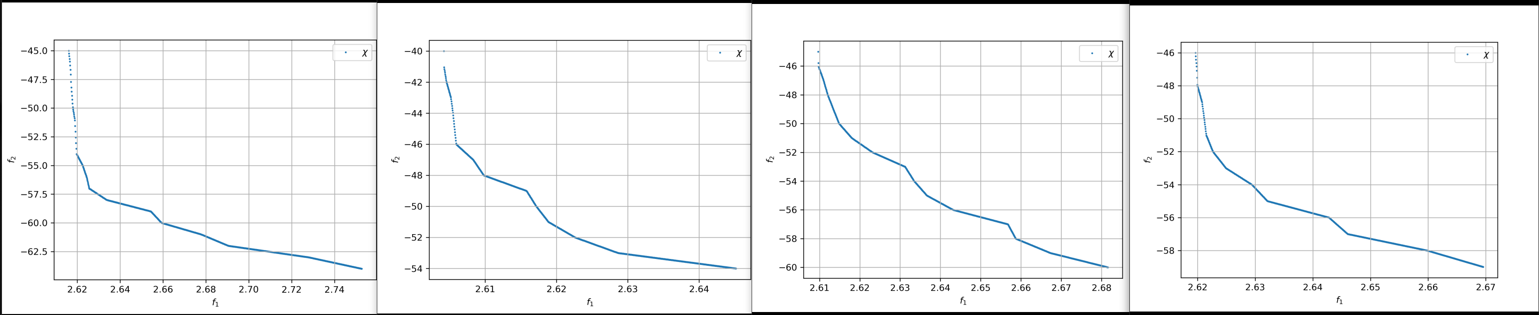
These results are still far from what fcmaes MODE (modecpp) can do in only 1600 seconds with DE update. But with NSGAII update, the results are quite consistent. Here are 4 modecpp runs with NSGA update using population size 768, each taking about 40 minutes:

Conclusion

The comparison with the results of Large Scale Discrete Constrained Black Box Optimization Using Radial Basis Functions is not intended to be "fair" if you compare only the number of objective function evaluations. The point is different:

The Mazda benchmark function, when called as a shared library and evaluated in parallel instead of via the command line, can be executed several thousand times per second. In that setup, it is not expensive to execute.
Once this is exploited, optimization algorithms that can handle many parallel function evaluations can "solve" the benchmark, both for the single-objective and the multi-objective case.
The Mazda benchmark’s collision analysis already uses a kind of domain-specific surrogate / approximation, which makes a very expensive generic surrogate-based method largely useless for this problem.

This should motivate looking for better implementations, parallelization, or clustering before using generic surrogate-based methods. Those methods often do not scale well to higher evaluation budgets and are often slow to execute. Simple changes such as:

Calling a library via ctypes instead of using the command line.
Using Numba for objective functions coded in Python.
Utilizing all threads of a modern many-core-CPU properly: Make sure the used method scales well with the number of cores used.
Creating a domain-specific "surrogate" approximating costly simulations to be used for global optimization.

can cause a dramatic speedup. Large Scale Discrete Constrained Black Box Optimization Using Radial Basis Functions reports 21 minutes for 4440 function evaluations even without using the expensive generic surrogate. That is a factor > 1000 compared to our implementation. Note that both are based on the same unmodified Mazda benchmark code implemented in C++.