

Robot Pushing and Navigating Rovers
This tutorial covers two real-world optimization benchmarks: robot pushing and rover navigation. Both are adapted from Bayesian test functions, which were originally created to evaluate an advanced Bayesian optimizer.
Motivation
Bayesian optimizers often perform well during the first few thousand objective evaluations. This is visible in the results reported in Wang 2018. But there are important drawbacks:
-
The optimizer itself has high overhead. For large-scale BO, kernel learning dominates the compute cost.
-
Reported research results usually focus on the number of evaluations, not on parallel execution.
-
Scaling gets worse as the evaluation budget increases.
To evaluate the practical value of Bayesian optimization on these two problems, we measure how long it takes to surpass the best results reported in Wang 2018 when all parallel threads of a modern multi-core CPU (AMD 5950x) are used. In both cases, this takes only a few seconds on a single CPU. Wang 2018 states: "EBO uses 240 cores via the Batch Service of Microsoft Azure", although it is not clear whether this setting was used for these two problems.
Optimizing the trajectory of a rover
The code for this example is at rover.py (adapted from Bayesian test functions). It implements a 60-dimensional trajectory optimization task in 2D that emulates rover navigation. See Wang 2018 for more details.
To use the 32 parallel threads of the AMD5950x efficiently, it is best to run parallel retries of the whole optimization:
-
Objective function evaluation is cheap, so 32 optimizations can run in parallel with little overhead.
-
This improves convergence reliability.
-
The fcmaes DE algorithm also supports parallel function evaluation, but this approach does not scale as well with thread count.
We execute 20 runs each with the fcmaes DE and BiteOpt algorithms using a limited evaluation budget.
from fcmaes.optimizer import De_cpp, Bite_cpp, wrapper, logger
from fcmaes import retry
from scipy.optimize import Bounds

...

    f_max = 5.0
    f = ConstantOffsetFn(domain, f_max)
    f = NormalizedInputFn(f, raw_x_range)
    x_range = f.get_range()

    bounds = Bounds(x_range[0], x_range[1])

    def negated(x): # negation because we minimize
        return -f(x)

    logger().info("rover retry.minimize(wrap(f, dim), bounds, De_cpp(10000), num_retries=32)")
    for i in range(20):
        retry.minimize(wrapper(negated), bounds, optimizer=De_cpp(10000), num_retries=32)

    logger().info("rover retry.minimize(wrap(f, dim), bounds, Bite_cpp(10000), num_retries=32)")
    for i in range(20):
        retry.minimize(wrapper(negated), bounds, optimizer=Bite_cpp(10000), num_retries=32)
We plotted the results of all 40 runs. Each run performs 32 parallel optimizations. For each run, only the best result across the parallel optimizations is shown.
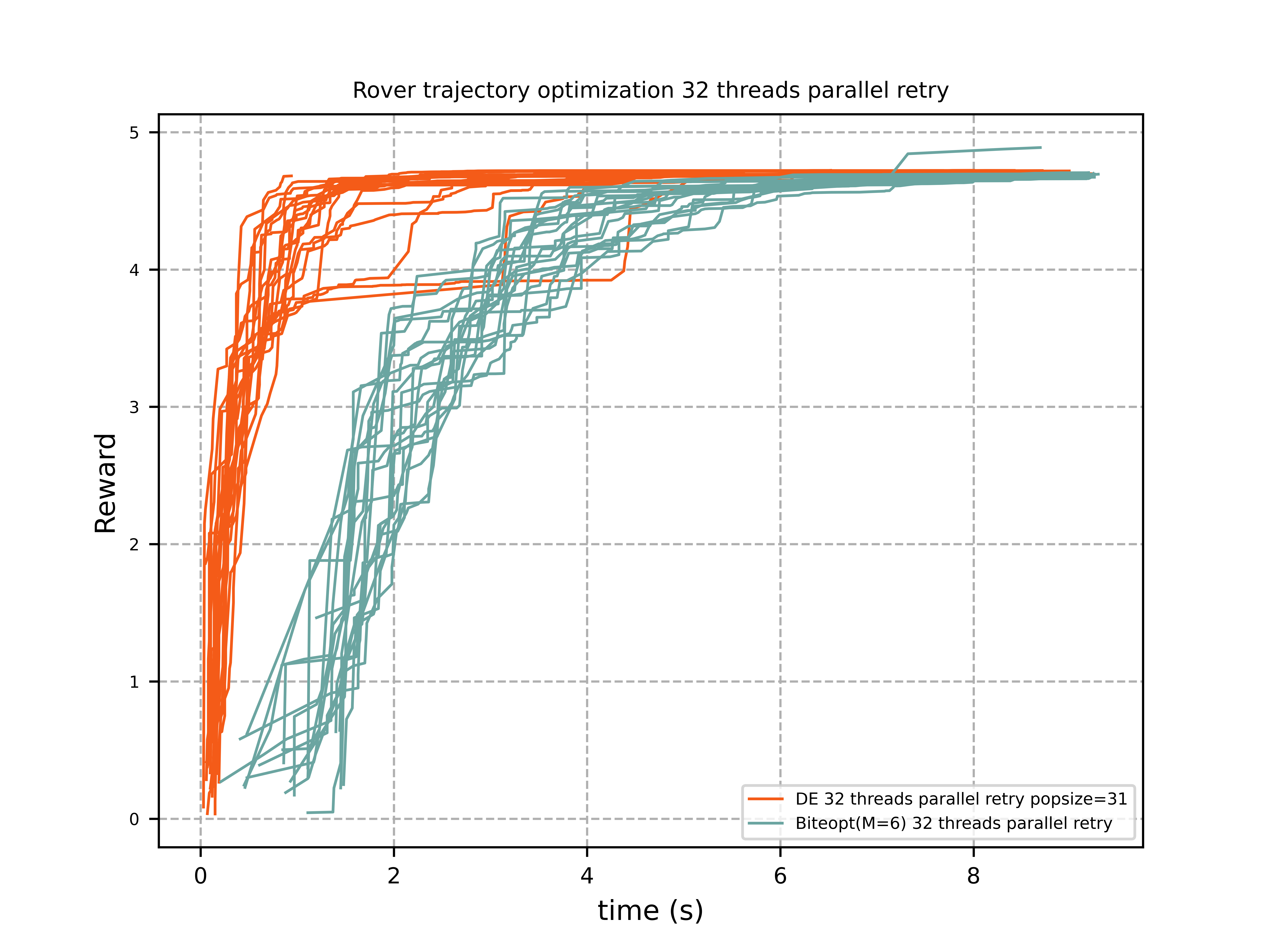
Wang 2018 reports CEM and EBO results below 4.0. As the diagram shows, none of the 40 experiments needed more than 5 seconds to improve on 4.0. All 40 runs converged to a result > 4.7 after 8 seconds.
Looking more closely at the diagram, BiteOpt produced a single outlier that was hard to reproduce. fcmaes provides a special meta-algorithm for such cases: smart boundary management. Even with that, you still need patience and luck.
    from fcmaes import advretry
    advretry.minimize(wrapper(negated), bounds, num_retries=10000, max_eval_fac=5)
Using this, we found a solution with reward = 4.922955944784702.
x = [0.08758383922294699, 0.28777608968376023, 0.37328808895554505, 0.0043381587210094795, 0.5383500175857339, 0.3510703935822824, 0.0030455390115092205, 0.8648400280085118, 0.07811932333841023, 0.5460177920661256, 0.4905636539961319, 0.7649544294506356, 0.2881006294931306, 0.7530736569481544, 0.5290621252472553, 0.9808427006512184, 0.5844194042218169, 0.8105477496464752, 0.6376884704466743, 0.7673028267533775, 0.7858470312335528, 0.4253686398575787, 0.1629990874037975, 0.808059766956296, 0.920883548506546, 0.9950223403480997, 0.8359973409613228, 0.8265379456184525, 0.9592582347752052, 0.9410315127889962, 0.3533737906965529, 0.9865294145252513, 0.8319077595955651, 0.6001369012272951, 0.4401274229007553, 0.9659369478713423, 0.3163442168705767, 0.7947645974747063, 0.8637257175268558, 0.9668728752424104, 0.766022487783223, 0.8740175737977381, 0.5684345360258591, 0.6238959237463229, 0.18820124840423424, 0.39049473247972066, 0.8387313390289421, 0.8932401812171913, 0.918259744546493, 0.786097201524139, 0.8460110243542978, 0.854774393702024, 0.7860576966000867, 0.8890763440050662, 0.9980659011537129, 0.4324613479054223, 0.8087367751757639, 0.9451787277717226, 0.7748986740730587, 0.9931182529188718]Finding a solution with reward > 4.9 is one of the hardest single-objective problems I have encountered.
What about the competition ?
There are not many open-source optimization libraries that match fcmaes in their support for parallelization, multiple objectives, and constraints. pymoo is one of them. It has excellent documentation and is easy to use. Here is the code to apply it to the rover trajectory problem. Check https://pymoo.org/algorithms/index.html for a list of alternative algorithms. The PSO algorithm has a useful animation feature that generates a video of the optimization progress. Unfortunately, PSO does not seem well suited to the rover trajectory problem.
    from fcmaes.optimizer import wrapper
    from pymoo.core.problem import ElementwiseProblem
    from pymoo.algorithms.soo.nonconvex.de import DE
    from pymoo.algorithms.soo.nonconvex.ga import GA
    from pymoo.algorithms.soo.nonconvex.pso import PSO
    from pymoo.factory import get_termination
    from pymoo.core.problem import starmap_parallelized_eval
    from multiprocessing.pool import ThreadPool
    import multiprocessing

    f_max = 5.0
    f = ConstantOffsetFn(domain, f_max)
    f = NormalizedInputFn(f, raw_x_range)
    x_range = f.get_range()

    def negated(x): # negation because we minimize
        return -f(x)

    class MyProblem(ElementwiseProblem):

        def __init__(self, **kwargs):
            super().__init__(n_var=len(x_range[0]),
                             n_obj=1,
                             n_constr=0,
                             xl=np.array(x_range[0]),
                             xu=np.array(x_range[1]), **kwargs)

        def _evaluate(self, x, out, *args, **kwargs):
            out["F"] = wrapped(x)

    pool = ThreadPool(32)
    #pool = multiprocessing.Pool(32)

    problem = MyProblem(runner=pool.starmap, func_eval=starmap_parallelized_eval)

    algorithm = DE(
        pop_size=100,
        #sampling=LHS(),
        variant="DE/rand/1/bin",
        CR=0.3,
        dither="vector",
        jitter=False,
    )

    algorithm2 = GA(
        pop_size=100,
        eliminate_duplicates=True)

    algorithm3 = PSO()

    res = minimize(problem,
                   algorithm,
                   #callback=PSOAnimation(fname="pso.mp4", nth_gen=5)
                   get_termination("n_gen", 1000000),
                   seed=1,
                   save_history=True,
                   verbose=False)
You can easily find a reward = 4.7 solution with this setting.
Although pymoo supports parallel function evaluations, that support is limited.
Using pool = multiprocessing.Pool(32) resulted in an
"AttributeError: Can’t pickle local object 'check_pymoo.<locals>.MyProblem" exception.
As a result, pymoo executes only about 2000 evaluations per second on the AMD5950 16-core processor,
instead of about 20000.
There is no support for parallelized optimization runs. You need a few retries to overcome the local minimum
at reward = 3.95. Note that pymoo’s Differential Evolution is quite different from the one in fcmaes.
It needs parameter fine-tuning and the right population size setting.
With the settings above, it needs about 30 seconds to find a reward = 4.7 solution, if it succeeds.
Optimizing the control parameters for robot pushing
The code for this example is at robot.py (adapted from Bayesian test functions). It implements a 14-dimensional control parameter tuning problem for robot pushing using fcmaes. See Wang 2018 for more details.
We switched off the GUI animation (do_gui=False) to speed up function evaluation, but it can be switched on to
visualize the optimization result.
Before executing the example code on anaconda please do:
-
pip install more-itertools
-
pip install pygame
-
conda install swig
-
pip install box2d-py
We again execute 20 runs each with the fcmaes DE and BiteOpt algorithms using a limited evaluation budget. As in the rover example, we use parallel retry for the same reasons:
from fcmaes.optimizer import De_cpp, Bite_cpp, wrapper, logger
from fcmaes import retry
from scipy.optimize import Bounds

...

    f = PushReward()
    bounds = Bounds(f.xmin, f.xmax)

    logger().info("push retry.minimize(wrap(f, dim), bounds, De_cpp(10000), num_retries=32)")
    for i in range(20):
        retry.minimize(wrapper(f), bounds, optimizer=De_cpp(10000), num_retries=32)

    logger().info("push retry.minimize(wrap(f, dim), bounds, Bite_cpp(10000), num_retries=32)")
    for i in range(20):
        retry.minimize(wrapper(f), bounds, optimizer=Bite_cpp(10000), num_retries=32)
We plotted the results of all 40 runs. Each run performs 32 parallel optimizations. Again, only the best result across the parallel runs is shown.
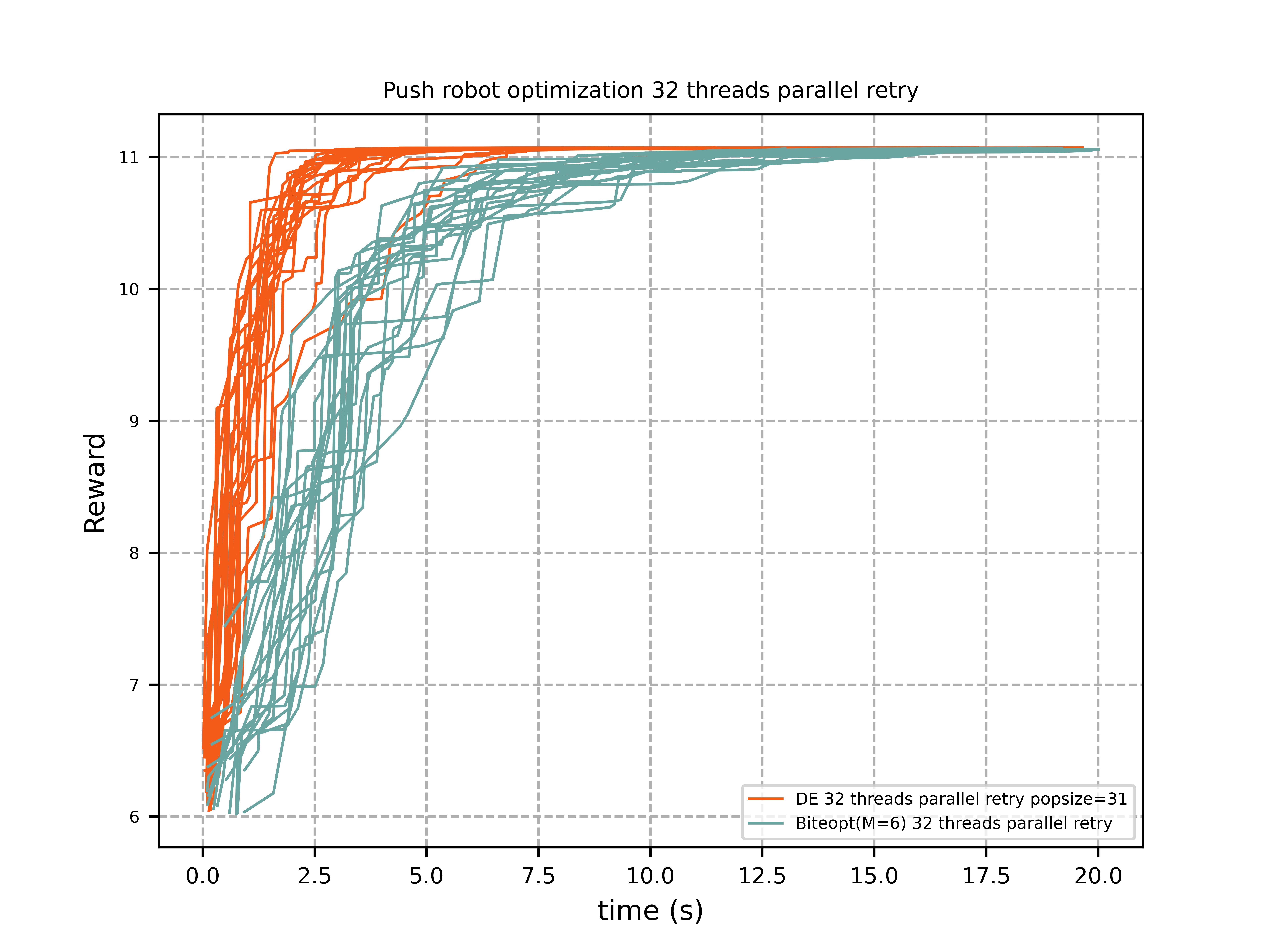
Wang 2018 reports: "CEM achieved a maximum reward of 10.19 while EBO achieved 9.50". As the diagram shows, none of the 40 experiments needed more than 7 seconds to improve on the CEM result (10.19). All 40 runs converged to a result > 11 after 20 seconds.
Conclusion
Neither the robot pushing problem nor the rover trajectory problem makes a strong case for advanced Bayesian optimization methods such as EBO (Ensemble Bayesian optimization) or CEM (noisy cross-entropy method), even though Wang 2018 shows that they are much better than other Bayesian methods such as BO-SVI and BO-Add-SVI. In both examples, fcmaes parallel retry with either Differential Evolution or BiteOpt finds better solutions within a few seconds.