fcmaes - a Python 3 gradient-free optimization library

Map Elites

This tutorial

Shows how to apply QD algorithms (Quality Diversity) to a space-flight planning problem with an extremely rugged solution landscape and a huge number of local optima.
Discusses how different configurations and solution emitters affect the result.
Explains how CVT MAP-Elites can be implemented in Python with low algorithm overhead and good scaling across parallel processes.
Shows how CMA-ES can improve optimization results further or refine existing solutions.

Remark

If you just want to try QD algorithms, start with the simple example arm.py, a simulation of a planar robot arm. Change the parameters and algorithms to see how they behave. The problem discussed here is "special" because the solution landscape is extremely rugged. For most other problems we recommend the fcmaes diversifier QD meta-algorithm, see Diversity.adoc. As shown below, diversifier also works well for the problem discussed here.

Background

Back in 2015, an influential book was published: Why Greatness Cannot Be Planned: The Myth of the Objective, review. It sparked a wave of research in quality diversity (QD). See Overview QD, Papers QD and Map-Elites-Overview.

QD algorithms often find better global solutions than traditional methods that are built to return a single optimum. Gradients can help, but they also lead into dead ends. The fcmaes library already leans toward diversity because it avoids gradients and uses a parallel retry mechanism. Still, it did not include a dedicated QD algorithm. I recently spent more time on the topic to see whether QD algorithms are mature enough for very hard optimization problems, including ESA’s GTOP problems, where they had not been applied before.

Note that fcmaes is mainly aimed at problems with dimension ⇐ 1000. Optimizing neural networks may require many thousand decision variables and is better suited to GPUs or TPUs. You may want to try evojax map_elites or evojax diversifier, which is derived from fcmaes diversifier.

Motivation

Let us start with an example. Suppose we are planning a space exploration mission to Saturn. As long as we cannot produce propellant in space, escaping Earth’s gravity remains very expensive. We therefore want to use gravity assists from planets along the way to reduce fuel consumption.

There are simplified models for this kind of mission. ESA used one of them to define a 22-dimensional optimization benchmark. This model includes so-called deep space maneuvers and is accurate enough to produce meaningful results, even though it ignores solar wind and details of the three-body problem during planetary flybys.

The model is accurate enough to search for interesting planning alternatives. These can then be reviewed with additional criteria and passed into a more detailed planning and optimization process.

But there is a problem: ESA’s Cassini2 benchmark evaluates only a single optimization result. From a real-world perspective, that is of limited use:

The model is not accurate enough to prove that the displayed solutions are really optimal.
The benchmark does not require alternative solutions for the planning process.

So what do we actually learn from the benchmark results?

The problem is hard. It took more than a year to find the optimal solution back in 2009.
We get a "reference solution" that can be used to compare methods and algorithms.
There is some diversity because six different teams produced slightly different results. But if you need 100 alternatives, do you really want to hire 100 teams?

You can try random solutions, which produces beautiful pictures like

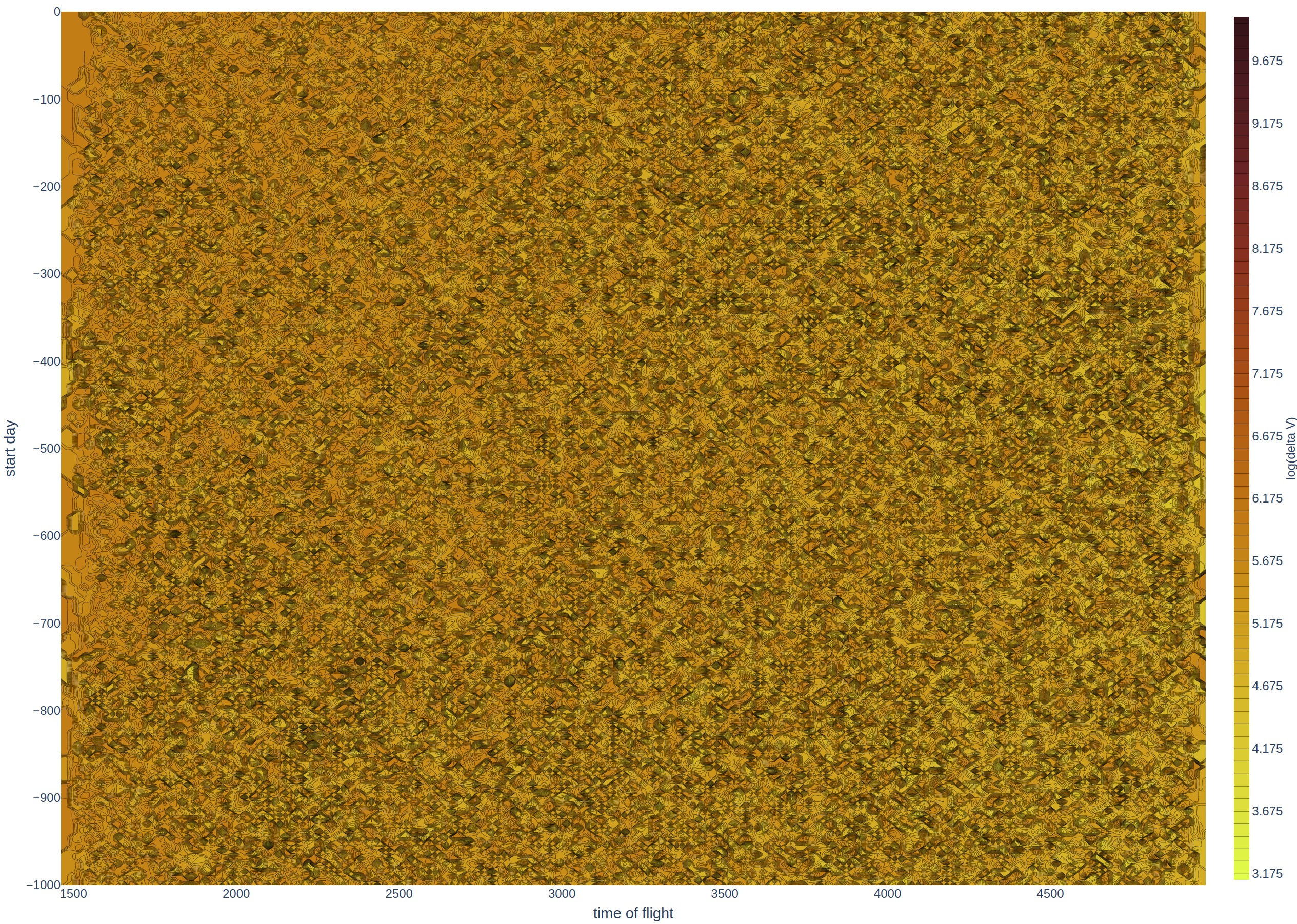
if you use a billion of them. But even the best random solutions still miss the global optimum by a factor of 2.8. Even a billion random samples do not reveal the promising regions in the two-dimensional feature space of start time and time of flight. A QD algorithm can produce a picture like

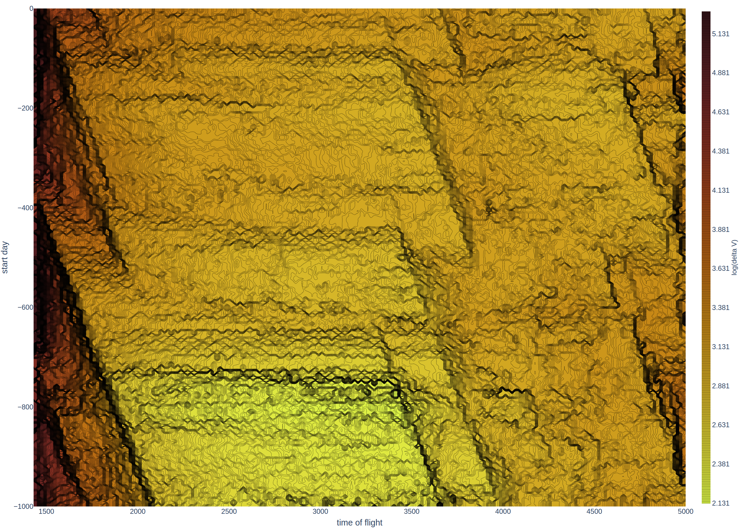
where we can clearly see that a start around day -800 is promising, and that flight times shorter than 1900 days or longer than 3500 days make little sense.

Planning Goal

As a mission planner, what do we actually want from an optimization algorithm? Something like this:

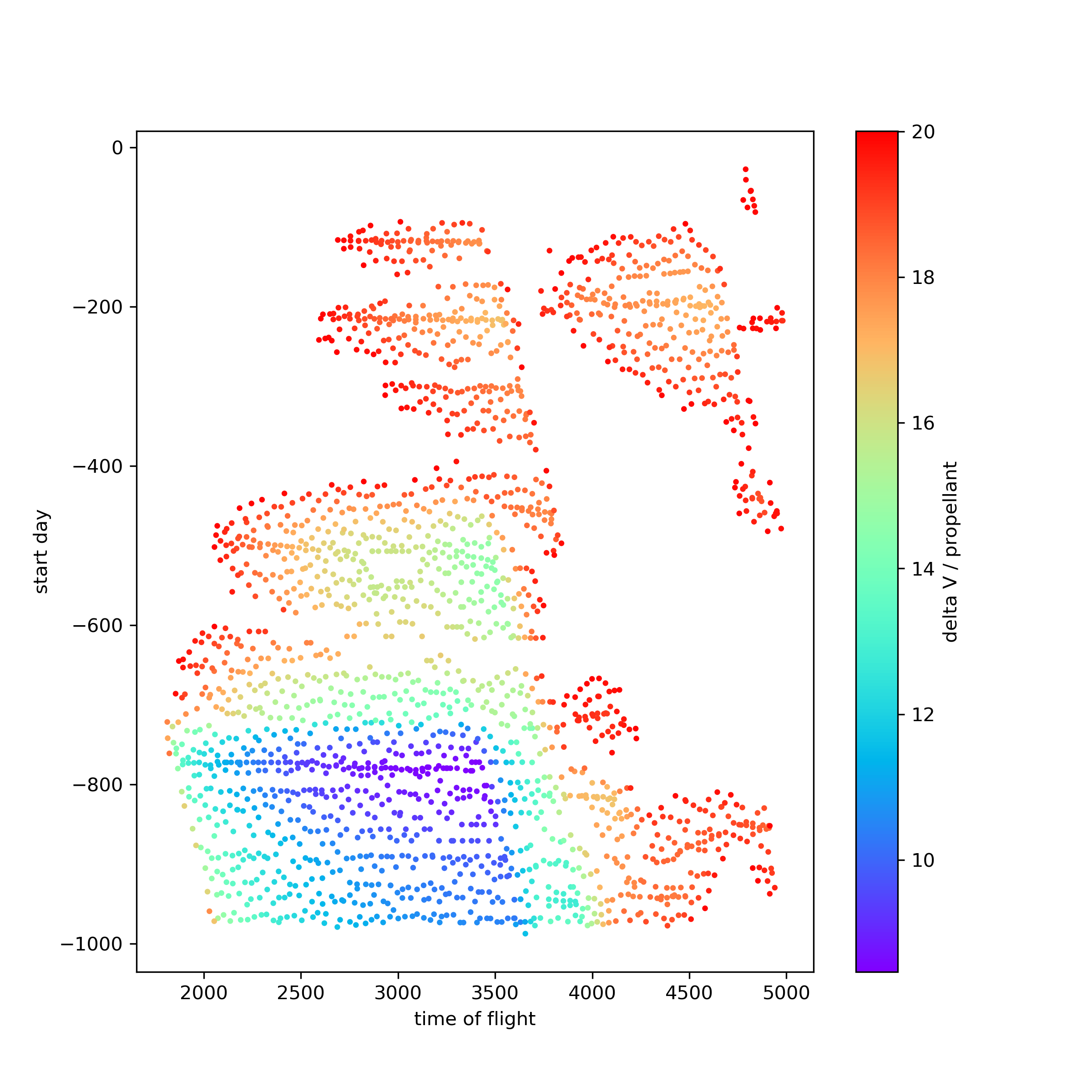
The diagram above shows 2159 different solutions to the Cassini2 problem with a fitness value ⇐ 20. For Cassini2, the fitness value is proportional to the propellant or fuel required for the whole mission. We can clearly see which mission start days and total mission times provide valid planning alternatives. The global optimum around 8.4 is also included. So even though we computed many alternatives, we still found the absolute optimum.

Next, we would like a fast preview that looks like this:

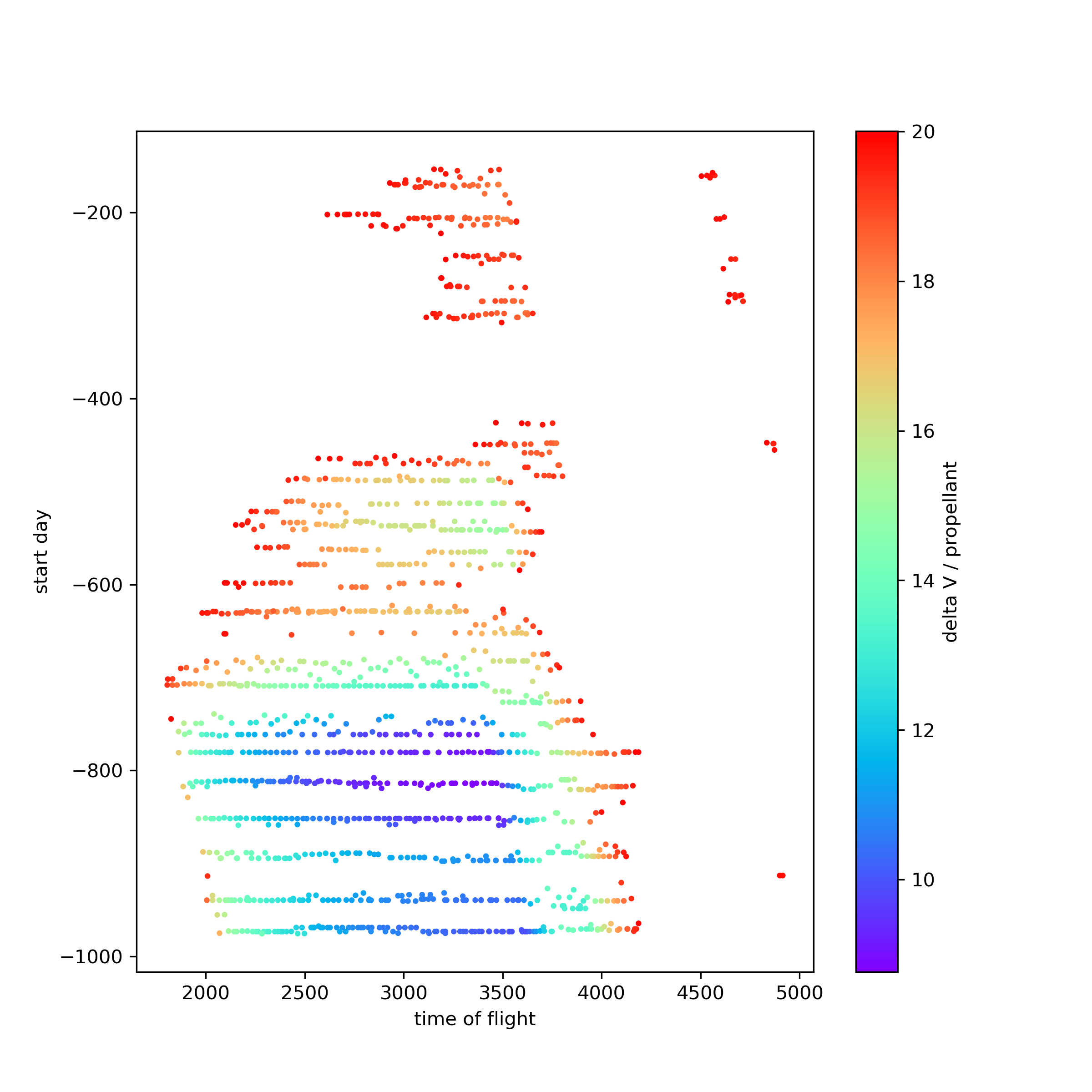
This preview contains fewer good solutions (1391), but it took only about 12 minutes on a modern 16-core desktop CPU. The good solutions appear in very similar regions, only their fitness values are slightly worse. Whether we really need the refinement shown above is debatable. The model itself has clear limits, and the preview already captures most of the best planning options around the global optimum.

Existing Python Implementations

The Cassini2 benchmark is implemented in C++ and wrapped in a Python API. Existing Python implementations do not cover this use case well for two main reasons:

The C++ wrapper causes problems for the usual Python parallelization approach because serialization fails when objects are transferred between processes.
If only individual fitness calls are parallelized, the overhead is larger than the gain for very fast fitness functions such as Cassini2.

It is possible to overcome these issues in Python, but it requires a different inter-process communication model. fcmaes already uses one for parallel optimization, based on shared memory.

Fortunately, the "fast preview" use case is already covered by CVT Map Elites, which also comes with a Python reference implementation.

We can also learn how to build an "afterburner" that improves existing solutions and can even expand the set of good solutions. CMA-ME, implemented here, integrates CMA-ES with MAP-Elites. Here we can find a JAX-based implementation that runs on GPUs and TPUs.

The main ideas behind these methods are:

The fitness function must also return a behavior or descriptor vector. It describes features of a solution that we want to distinguish, for example "start day" and "time of flight" for Cassini2.
Voronoi tessellation is used to divide the behavior space into niches. This still works for higher-dimensional behavior spaces. Experiments with Cassini2 show that it is advantageous even with only two behavior dimensions.
CMA-ES is adapted by sorting solutions not by raw fitness, but by the fitness difference to the current elite of the corresponding niche. Since this sorting drives the search-space reshaping in each generation, it encourages the algorithm to search for new solutions.

But what if the model used for optimization is not fully accurate, as in ESA’s Cassini2 benchmark? Then it may not be worth spending too much time polishing existing solutions. A better strategy is often to filter the solutions with a more accurate model, or with additional criteria and constraints. Only the filtered solutions would be carried forward and possibly optimized further.

Existing algorithms do not support this use case, so we created a new one. We still apply CMA-ES, but this time we modify the fitness differently:

We use the new fitness function returning the behavior vector.
But instead of returning it we check if we are still in the initial niche.
If yes, we return the fitness value, if not we return infinity.
Additionally we restrict the box boundaries: We use the minimal/maximal values of the decision variable values for all fitness computations executed during the preliminary Map-Elites run associated with the niche we optimize.

For Cassini2 this method works quite well when improving a specific selection of niches.

Multi Modal Optimization Problems

Most real-world optimization problems are multi-modal. They have many local minima:

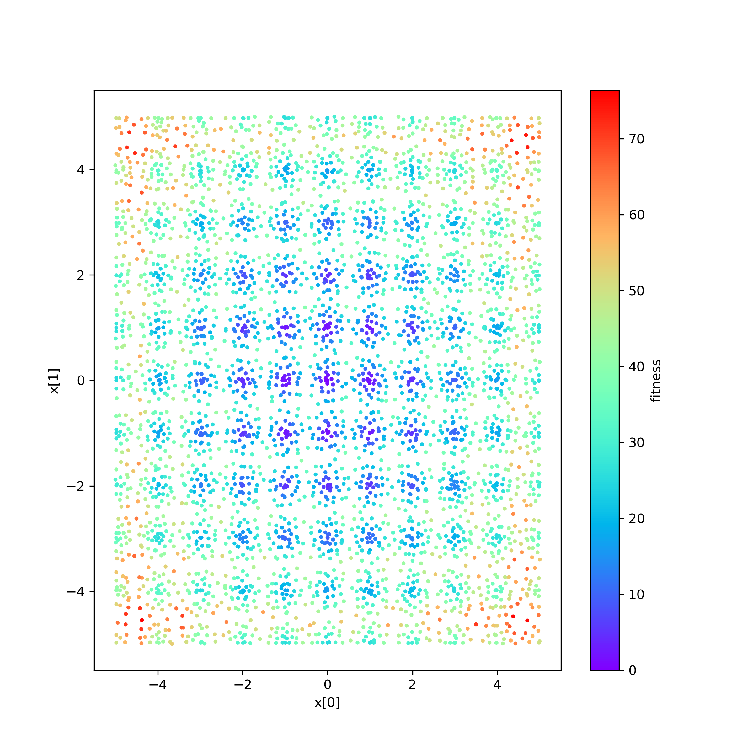
Often we do not want only the single best solution. We also want to understand the alternatives. The picture above plots the first two dimensions against the fitness value for the 10-dimensional rastrigin function. You cannot easily enumerate a complete grid of solution variables because the size of such a grid grows exponentially with the number of decision variables. But you can generate millions of random solutions and use these:

from numpy.random import default_rng
from numba import jit
import numpy as np
import math

@jit
def rastrigin(x):
    return 10 * x.shape[0] + (x * x - 10 * np.cos(2 * math.pi * x)).sum()

def random_test(dim = 10, rng = default_rng()):
    xs = rng.uniform(np.full(dim, -5), np.full(dim, 5), (10000000, dim))
    best = math.inf
    for x in xs:
        y = rastrigin(x)
        best = min(y, best)
    print(best)

Note: Never forget to use numba or JAX to speed up your fitness function if you do not want to wait forever.

With this approach you usually get a best fitness somewhere between 30 and 40. The picture above was generated with a better method. In many real-world problems, the number of evaluations is limited even if you use all available CPU cores. To analyze the optimization result, we can also use a 3d view:

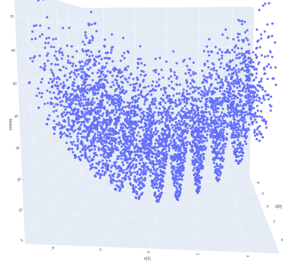
This 3d representation is easier to analyze interactively from different angles. The key questions are:

Is there a method that can explore a complex multi-modal fitness function and still capture the local minima correctly?
Can it find the global optimum?
Does it work for complex real-world applications?

All of these questions are addressed below.

Multi-objective optimization

One way to approach the problem is to apply multi-objective optimization and use the x- and y-axis as additional objectives:

from scipy.optimize import Bounds
from fcmaes modecpp

@jit(cache=True,fastmath=True)
def rastrigin_mo(x):
    return x[0], x[1], 10 * x.shape[0] + (x * x - 10 * np.cos(2 * math.pi * x)).sum()

def mo_test(dim = 10):)
    bounds = Bounds(np.full(dim, -5), np.full(dim, 5))
    xs, ys = modecpp.retry(rastrigin_mo, 3,
                0, bounds, num_retries=32, popsize = 1000, max_evaluations = 5000000, workers=32)

Because fcmaes multi-objective optimization scales well with the number of cores, on a modern 16-core CPU such as the AMD 5950x we can execute 32x5000000 evaluations in less than one minute and get the following picture:

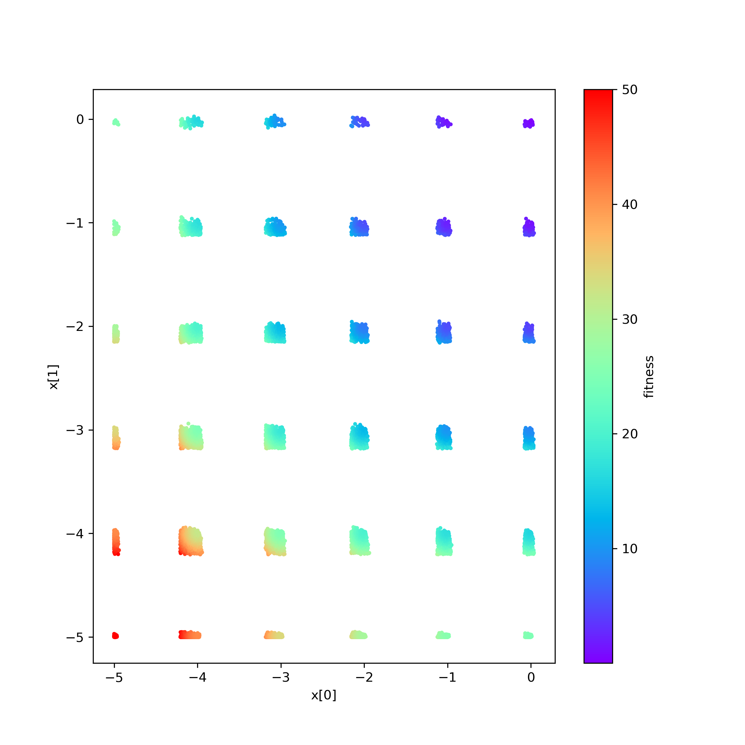
The problem is obvious. The global optimum was found, but we only see one quadrant of the real solution set. What happened? By defining x[0] and x[1] as additional objectives, we told the algorithm to prefer solutions with lower x[0] and x[1] values. The Pareto-front computation then eliminated all dominated solutions, so we only see solutions with negative x[0] and x[1].

If that bias is not intended, we need another approach:

Map-Elites

A few years ago, a new approach to this problem was proposed: Map Elites.

In Map-Elites, the fitness function returns not only a fitness value, but also a list of "behavior/descriptor" values that enforce solution diversity. We want to find good solutions and local minima for different "descriptor" values:

def fitness_me(x):
    ...
    return fitness, np.array[descriptor1, descriptor2, ...]

In the rastrigin examples above, the descriptor values are x[0] and x[1], which are used as the x- and y-axis of the plots. The descriptor vector usually has lower dimensionality than x, so it is easier to tessellate into separate cells. Map-Elites is a well-known QD (Quality-Diversity) algorithm and works as follows:

Tessellate the descriptor space into n cells called archive.
Initialize each archive cell with a random solution and assign math.inf as fitness value.
Generate candidate solutions by crossover, mutation, or other methods based on a random selection of solutions from the archive.
Evaluate the candidates and determine their descriptors by applying fitness_me.
For each candidate determine its cell and replace its content if the candidate improves on the incumbent.

But what if we have more than two descriptor dimensions? Then the "curse of dimensionality" appears here as well, and tessellation becomes less trivial. Fortunately CVT Map Elites solves this issue by using Voronoi tessellation. Even better, there is a reference implementation.

Performance Comparison

cvt_rastrigin.py already provides the 10-dimensional rastrigin example shown above. For our experiments, we reduce the number of archive cells to n_niches=4000, because otherwise the algorithm is dominated by the cost of finding the cell for a descriptor vector. We increase px["dump_period"] = 10000000 to avoid file writes during optimization. We then benchmark the optimization itself, excluding the initialization and archive creation phase. We test both px["parallel"] = False and px["parallel"] = True, and both regular fitness and numba/@jit.

Table 1. Fitness evaluations per second rastrigin
	parallel=False @jit off	parallel=False @jit on	parallel=True @jit off	parallel=True @jit on
reference implementation	11527	13526	9480	9632
fcmaes Map-Elites	64214	90577	755254	950557

Comparing the best setting of each implementation gives 950557 / 13526 = factor 70 speedup. This comes from lower algorithm overhead and much better scaling under parallelization.
Parallelization reduces performance for the reference implementation.
In single-threaded mode we still get 90577 / 13526 = factor 6.7 speedup, caused by lower algorithm overhead alone.

The reference implementation handles parallelism with multiprocessing.Pool.map:

def parallel_eval(evaluate_function, to_evaluate, pool, params):
    if params['parallel'] == True:
        s_list = pool.map(evaluate_function, to_evaluate)
    else:
        s_list = map(evaluate_function, to_evaluate)
    return list(s_list)

This has several disadvantages:

A separate parallel call for each fitness evaluation adds a lot of overhead.
multiprocessing.Pool.map uses serialization and pickle to transfer data and relies on locks to avoid conflicting access.
Serialization causes problems for closures and functions that call C code.
Locks are not needed if communication is implemented with shared memory, as fcmaes does.

fcmaes instead processes whole chunks of fitness evaluations inside the same process, which reduces overhead.

We performed another test with a much more expensive fitness evaluation:

Table 2. Fitness evaluations per second expensive fitness
	parallel=False @jit off	parallel=True @jit off
reference implementation	12.6	200.6
fcmaes Map-Elites	17.0	304.8

As expected, the disadvantage of using multiprocessing.Pool.map becomes much smaller in this case.

You may argue that real-world fitness functions are often expensive. Examples are the complex simulations used in the FluidDynamics and PowerPlant tutorials. But these expensive real-world fitness functions also do not survive the serialization done by multiprocessing.Pool.map. And in many of the other tutorials, fitness evaluation is very fast once we use numba or implement it directly in C.

Space flight mission design

We will use ESA’s Cassini2 Mission design benchmark, already discussed in SpaceFlight.

It models the planning of a mission to Saturn with several planetary gravity-assist maneuvers. The simplified model includes the start time and velocity, the timings between planets, the flyby height and angle, and the timing of the deep space maneuvers between planets.

Let us first look at the original benchmark. It uses a fixed planet sequence and requires 22 decision variables. Although it is not the hardest of the GTOP problems, it is still difficult to solve, even if you only care about the global optimum.

Meaningful Map-Elites descriptors are the mission start time and the overall time of flight, because those are the mission options we want to inspect. Note that there is a clear preference for earlier starts and shorter flight times, so multi-objective optimization with the descriptors as additional objectives is also a valid alternative here.

CVT MAP-Elites doesn’t work for ESAs Cassini2 benchmark

Let us first try the Python reference implementation of CVT MAP-Elites. We need to normalize both the solutions and the behavior descriptions, but otherwise the setup is straightforward. We use an fcmaes fitness wrapper to monitor progress and measure the evaluation rate.

import map_elites.cvt as cvt_map_elites
import map_elites.common as cm_map_elites
from fcmaes.astro import Cassini2
from fcmaes.optimizer import wrapper

problem = Cassini2()
bounds = problem.bounds
px = cm_map_elites.default_params.copy()
px["dump_period"] = 2000000
px["batch_size"] = 200
px["min"] = 0
px["max"] = 1
px["parallel"] = False

fun = wrapper(problem.fun)

lb = bounds.lb
scale = bounds.ub - bounds.lb

def fitness(x):
    x = lb + np.multiply(x,scale)  # denormalize
    return -fun(x), get_tof_launch_time(x)

def get_tof_launch_time(x): # normalize
    tof = sum(x[4:9]) / 5000.0
    launch_time = (1000 + x[0]) / 1000.0
    return np.array([tof, launch_time])

def test_cassini2():
    archive = cvt_map_elites.compute(2, 22, fitness, n_niches=4000, max_evals=1e8, log_file=open('cvt.dat', 'w'), params=px)

if __name__ == '__main__':
    test_cassini2()

For the configured 1e8 evaluations, my machine (AMD 5950x) needs almost 4 hours. The best fitness value found is 10.85, and the optimization runs at 7150 fitness evaluations per second. That is far too slow to be useful. Apart from the speed, the reference implementation behaves as expected. For 1e8 evaluations this result is reasonable because we do not use CMA-ES here.

With px["parallel"] = True, the optimization slows down to about 4500 evaluations per second because the additional process creation overhead outweighs the benefit by far.

CVT MAP-Elites does work for ESAs Cassini2 benchmark

The code implementing CVT MAP-Elites optimization with fcmaes is here: elitescass2.py. It reaches up to 350000 fitness evaluations per second, which is about a factor of 50 faster. The speedup is a factor of 78 if you compare it with px["parallel"] = True. In addition, the CMA-ES emitter improves convergence, and we find solutions around 8.6 in about 15 minutes. The plots shown above display the whole archive, which contains a large number of good solutions. The code uses mapelites.py, the fcmaes CVT Map-Elites implementation.

...
def tof(x):
    return sum(x[4:9])

def launch(x):
    return x[0]

class Cassini2_me():
    ''' Map-Elites wrapper for the ESA Cassini2 benchmark problem'''

    def __init__(self, prob):
        ...
        self.bounds = prob.bounds
        min_tof = tof(prob.bounds.lb)
        max_tof = tof(prob.bounds.ub)
        min_launch = launch(prob.bounds.lb)
        max_launch = launch(prob.bounds.ub)
        self.qd_bounds = Bounds([min_tof, min_launch], [max_tof, max_launch])

    def qd_fitness(self, x):
        return self.problem.fun(x), np.array([tof(x), launch(x)])

def run_map_elites():
    problem = Cassini2_me(Cassini2())
    me_params = {'generations':100, 'chunk_size':1000}
    cma_params = {'cma_generations':100, 'best_n':200, 'maxiters':1000, 'miniters':200}
    fitness =  mapelites.wrapper(problem.qd_fitness, problem.qd_dim)

    archive = mapelites.optimize_map_elites(
        fitness, problem.bounds, problem.qd_bounds, niche_num = niche_num,
          iterations = 50, me_params = me_params, cma_params = cma_params)

Here, neither the solution space nor the descriptor space is normalized, so we have to provide the corresponding bounds to the algorithm (problem.bounds, problem.qd_bounds). Archive objects also have load and save methods, so the optimization state can be written to disk. A saved archive can be passed back to mapelites.optimize_map_elites through the optional archive parameter to continue an earlier run. The performance difference compared to the reference implementation has several reasons:

Although both implementations use sklearn.neighbors.KDTree to determine the niche, fcmaes forwards whole chunks of solutions to the KDTree, which speeds things up significantly.
fcmaes applies the same trick for SBX (Simulated binary crossover) and Iso+Line to avoid slow Python loops.
Because fcmaes stores the archive in shared memory, processes can evaluate many solutions before they have to synchronize. This greatly reduces process creation and shutdown overhead. Because of Python’s global interpreter lock, multithreading is not applicable here, and process creation is relatively heavyweight.
The reference CVT MAP-Elites implementation does not support CMA-ES updates, so there is no direct comparison for that part.

Because its covariance matrix update is computationally expensive, CMA-ES can become very slow for higher-dimensional solution spaces. The underlying matrix library may also allocate multiple CPU cores to a single optimization, which is counterproductive if the full optimization is already parallelized. For extremely high dimensions (> 1000), there is no real alternative to a JAX based implementation, where the matrix operations are delegated to a GPU or TPU. But as the benchmark results in EvoJax.adoc show, CMA-ES is usually not the best choice for such high-dimensional problems anyway because convergence is too slow. For MAP-Elites, which is usually applied to problems with dimension < 1000, a fast C++ CMA-ES implementation such as the one in fcmaes fits very well because it stays single-threaded and integrates cleanly with higher-level parallelization.

There is an alternative: Diversifier

diversifier.py is a newer alternative to MAP-Elites. It generalizes ideas from CMA-ME to other wrapped algorithms. It uses the archive from CVT MAP-Elites (https://arxiv.org/abs/1610.05729), implemented in mapelites.py.

There is also an equivalent implementation for the machine learning domain: evojax diversifier, which can handle many thousand decision variables. It parallelizes at a different level: in the fitness function and in the optimization algorithm itself.

Both the parallel retry mechanism and the archive-based modification of the fitness function improve the diversity of the optimization result. The resulting archive can be stored and used later to continue the optimization.

Like MAP-Elites, it requires a QD fitness function that returns both a fitness value and a behavior vector, which is used to determine the corresponding archive niche through Voronoi tessellation. It returns, or improves, an archive of niche elites and also stores statistics about the associated solutions for each niche.

def run_diversifier():
    name = 'cass2div'
    problem = Cassini2_me(Cassini2())
    opt_params0 = {'solver':'elites', 'popsize':1000, 'workers':16}
    opt_params1 = {'solver':'DE_CPP', 'max_evals':50000, 'popsize':31, 'stall_criterion':3}
    opt_params2 = {'solver':'CMA_CPP', 'max_evals':100000, 'popsize':31, 'stall_criterion':3}
    archive = diversifier.minimize(
         mapelites.wrapper(problem.qd_fitness, 2), problem.bounds, problem.qd_bounds,
         workers = 32, opt_params=[opt_params0, opt_params1, opt_params2], max_evals=2000000*32)
    diversifier.apply_advretry(wrapper(problem.fitness), problem.descriptors, problem.bounds, archive, num_retries=20000)
    archive.save(name)
    plot_archive(archive)

As the example code shows, it supports arbitrary combinations of solvers. Solvers are treated as a sequence, except for 'solver':'elites', which is executed in parallel. 'workers':16 means that 16 of the configured 32 parallel processes are allocated to MAP-Elites, and the rest to the other solvers. In a sequence, here DE → CMA-ES, the best solution found is passed to the next solver as the initial mean of its solution distribution. max_evals for diversifier.minimize limits the overall number of fitness evaluations. For the individual optimizers, max_evals limits the number of evaluations in a single optimizer run.

Note that the use of solver sequences is specific to space-flight planning tasks. In most cases, a combination of CMA-ES or CR-FM-NES and MAP-Elites running in parallel works very well.

A resulting niche archive may be improved further by applying a regular non-QD algorithm: the fcmaes advanced parallel retry and smart boundary management meta-algorithm. The archive contents are transferred to its solution store and then back to the QD archive. This method is very effective at improving the best solutions found so far, but it does not improve diversity very much.

The diversifier needs fewer fitness evaluations, at the price of some diversity. It can be an interesting alternative when the evaluation budget is limited or the fitness evaluation is expensive. Its results are still far more diverse than what can be achieved without a QD archive of niche elites.

Conclusion

We have shown that:

CVT MAP-Elites can handle even the hardest optimization problems.
QD algorithms are often more useful for real-world problems than optimizers that return only a single best solution.
The CMA-ES emitter improves existing archive solutions effectively during optimization.
CMA-ES can also be applied after MAP-Elites optimization to improve selected niches.
Alternatively, there is the general diversifier, which applies a QD archive to different non-QD algorithms such as CR-FM-NES, DE, PGPA, and CMA-ES, or to sequences of these. This flexibility is especially valuable in application domains where CMA-ES becomes slow, for example at dimension > 1000, as in many machine learning tasks.
QD archives and fcmaes parallel retry stores can exchange their solutions to improve results further using non-QD meta-algorithms.

Our CVT MAP-Elites implementation with CMA-Emitter, elitescass2.py, introduces several changes that improve performance:

Our archive uses shared memory to reduce inter-process communication overhead.
The initial behavior space is generated from uniform behavior samples because random solutions may cover only part of the behavior space. Some parts may become reachable only through optimization.
Fitness computations may be expensive. Therefore we avoid computing fitness values for the initial solution population.
The initial solution space is generated from uniform samples of the solution space. These samples are never evaluated. They serve as the initial population for SBX or Iso+LineDD, and their associated fitness value is set to math.inf. This has two effects:
- It avoids computing fitness values for the initial population.
- It increases the diversity of the initial solutions emitted by SBX or Iso+LineDD.
Iso+LineDD (https://arxiv.org/pdf/1804.03906) is implemented, but it does not work well with extremely ragged solution landscapes. Therefore SBX+mutation is the default setting.
SBX (Simulated binary crossover) is combined with mutation. Both spread factors, for crossover and mutation, are randomized for each application.
Candidates for CMA-ES are sampled with a bias toward better niches.
There is a CMA-ES drill-down mode for specific niches. In this mode all solutions outside the niche are rejected. Restricted solution box bounds are used, derived from the statistics maintained by the archive during the addition of new solution candidates.

Note that the Python reference implementation of CVT MAP-Elites also tessellates the behavior space independently of fitness evaluations of emitted solutions.