fcmaes - a Python 3 gradient-free optimization library

Space Flight Mission Design Revisited

This tutorial

Discusses a specific mixed integer multi-objective space flight dynamics problem and shows the results obtained with different methods.

Motivation

The initial development of fcmaes was driven by space flight mission design problems. Later, work on other real-world optimization tasks led to additional (meta-)algorithms. This tutorial closes that loop. It shows how these newer methods can be used for a specific multi-objective mission design problem.

Planning the Cassini Mission.

The original Cassini Mission to Saturn involved four gravity-assists at Venus, Venus, Earth and Jupiter to save fuel.

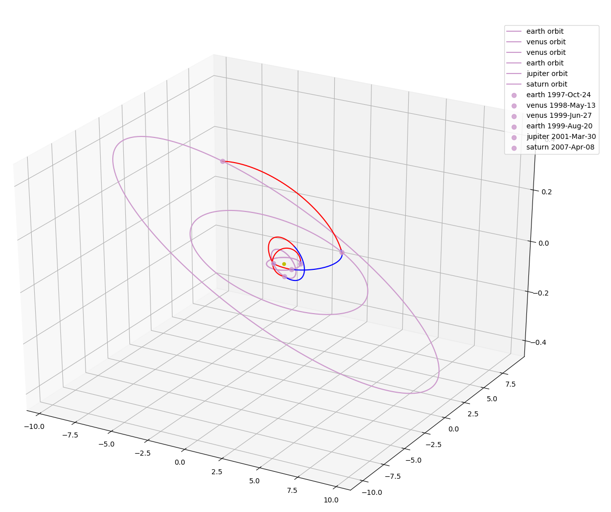
Now assume our task is to review that mission plan. The planning team used domain knowledge to decide which planets to visit and in which order. But can we trust that choice? To find out, we ignore their intuition and let the optimization select the route.

Optimizing Delta Velocity

Let us first look at the single-objective problem. The goal is to minimize fuel consumption, expressed as the sum of the delta velocities caused by the thrust impulses needed to navigate the spacecraft. Our first simplified flight model assumes that impulses are applied only at the planetary flybys, before and after the gravity assist (GA) maneuvers. Between planets, the spacecraft coasts. This reduces the problem to 10 decision variables: 6 for the flyby timings and 4 for the planets visited on the way. The fitness function truncates the float value to an integer. Here are the bounds for the decision variables:

    lb = [-1000.,30.,100.,30.,400.,1000., 2, 2, 2, 3],
    ub = [0.,400.,470.,400.,2000.,6000., 3.9999, 3.9999, 3.9999, 5.9999]

We restrict planet selection based on domain knowledge. For example, we do not want to visit Pluto on the way to Saturn. Note that the objective function rounds the planet choice to the next integer. The bounds are therefore defined so that each planet selection gets the same float interval.

    from fcmaes.astro import cassini1multi

    def cassini1(x):
        y = cassini1multi(x)
        return y[0]

    advretry.minimize_plot("cassini1_mixed bm", de_cma(1500), cassini1,
                               bounds, 10.0, 20.0, 5000, logger=logger())

Method cassini1 simply selects the first objective, delta velocity. We then apply the boundary management meta-algorithm (advretry) to perform a parallel retry of a DE→CMA-ES sequence.

Excercise: Try other (meta-)algorithms.

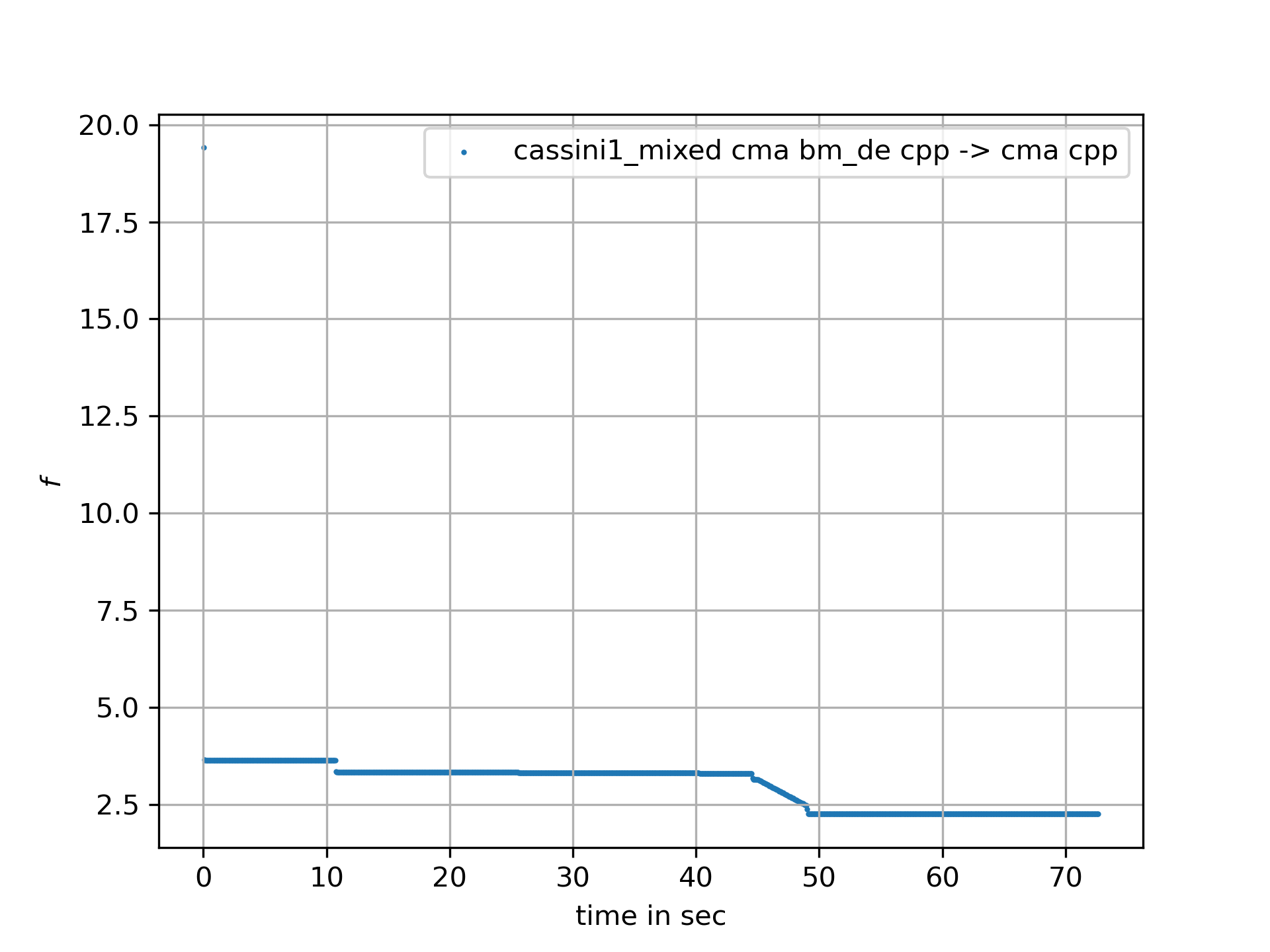
We quickly find solutions with the EVVE sequence and a suspiciously low dv of about 2.25 km/s. The planning team proposed a solution above 8 km/s. That means one of two things: either they missed a better planet sequence, or our model is too simple. We therefore try a more accurate model.

The new model allows one additional deep-space maneuver between two planets. This makes the problem much harder. We now have to decide at which angle and height the spacecraft passes the planets. That choice affects the trajectory change during the GA maneuver. The first model did not include this effect, because it could simply choose the local values that minimize delta velocity at the planet. In the new model, the same decision can have consequences several planets later.

lb = [-1000,3,0,0,100,100,30,400,800,0.01,0.01,0.01,0.01,0.01,1.05,1.05,1.15,1.7, -math.pi, -math.pi, -math.pi, -math.pi, 2, 2, 2, 3],
up = [0,5,1,1,400,500,300,1600,2200,0.9,0.9,0.9,0.9,0.9,6,6,6.5,291,math.pi,  math.pi,  math.pi,  math.pi, 3.9999, 3.9999, 3.9999, 5.9999]

The new model uses 26 decision variables: 22 for timings and flyby parameters, and 4 for the planet sequence.

    from fcmaes.astro import cassini2multi

    def cassini2(x):
        y = cassini2multi(x)
        return y[0]

    advretry.minimize_plot("cassini2_mixed bm", de_cma(1500), cassini2,
                               bounds, 12.0, 20.0, 20000, logger=logger())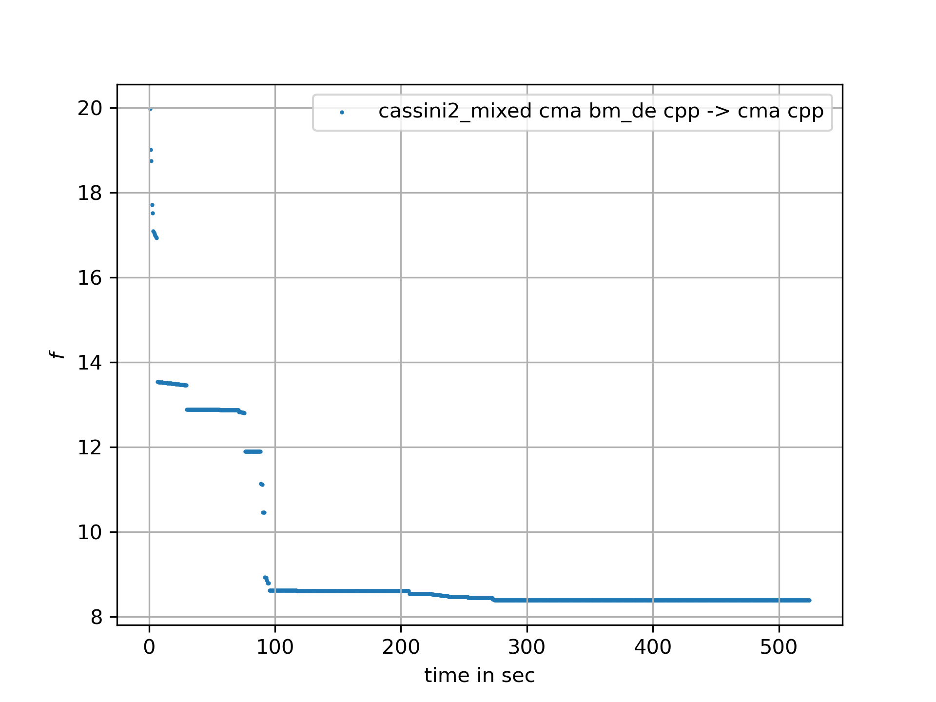

Now the selected tour is "VVEJ" with dv = 8.38, which matches the planning team’s proposal. So they were right after all, and the first model was indeed flawed. This problem is quite tough for optimization algorithms. Please notify me if you find one that solves it faster.

Optimizing Delta Velocity and Flight Time

Our boss storms into the office: "Almost ten years, this takes too long". She asks us to explore alternatives: "It’s ok if you need more delta velocity, we build a more efficient engine".

From the single-objective case we already know that we need the complex model with 26 decision variables, and that model is hard to solve. The second objective, TOF (time of flight), is derived directly from the decision vector. Experience shows that such an objective can easily dominate a multi-objective optimization. There is no single best algorithm for this kind of problem. Instead, we use several algorithms and combine the computed Pareto fronts.

We start with moretry.minimize. It applies the DE→CMA sequence using parallel retry, with different objective weightings for different runs. We weight the TOF objective much lower to compensate

for the effect that optimization "prefers" the objective which is more directly related to the decision variables
for the different scaling of the objectives (about 8 km/s, 2000 days)

    from fcmaes.astro import cassini2multi
    from fcmaes import mode, moretry

    def cassini2_2(x):
        y = cassini2multi(x)
        return y[:2]

    x, y = moretry.minimize(mode.wrapper(cassini2_2, 2, interval = 10000000),
             bounds, weight_bounds = Bounds([0.1, 0.001], [1, 0.001]),
             ncon = 0, value_exp = 2.0,
             num_retries = 50000, optimizer=de_cma(50000))
    np.savez_compressed("cassini2" + "de_cma50k", xs=x, ys=y)
    moretry.plot("cassini2" + "de_cma50k.5", 0, x, y, all=False, interp=True)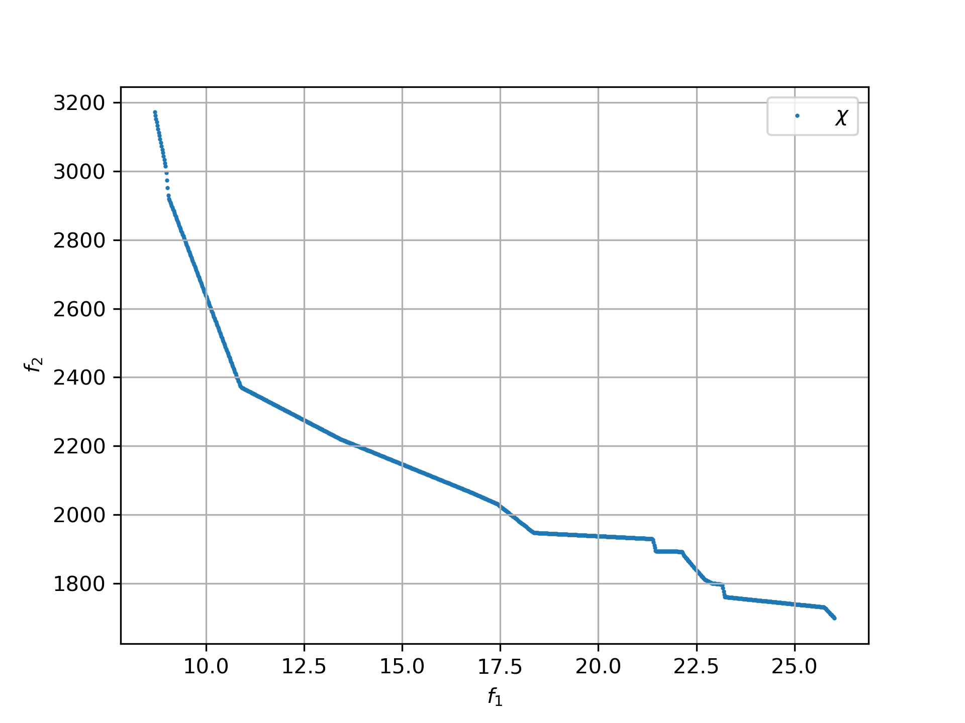

To complement this Pareto front, we use a real multi-objective algorithm: fcmaes MODE. To make good use of our CPU cores, we choose parallel retry instead of parallel function evaluation. This works well for objective functions that are fast to evaluate. modecpp.retry executes parallel runs of the MODE algorithm, in this case using NSGA-II population update.

  x, y = modecpp.retry(mode.wrapper(cassini2_2, 2, interval = 10000000), 2, 0,
                 bounds, popsize = 128, max_evaluations = 1000000,
                 nsga_update=True, num_retries = 256)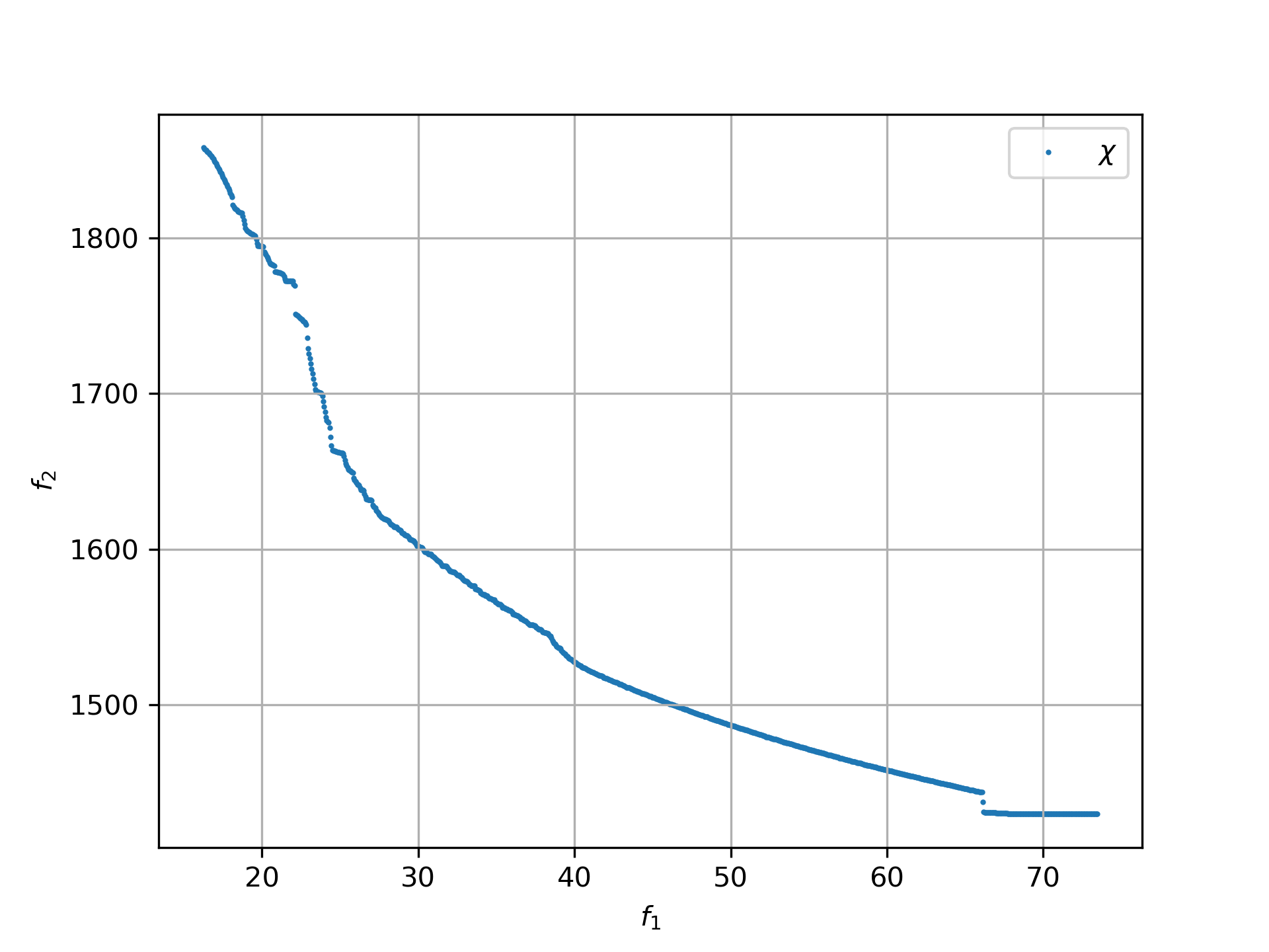

MODE does not find the very best low-DV solutions. This time, however, the high-DV region with dv > 20 km/s is covered much better. We find solutions with TOF < 1500 days, which was not possible with moretry.

Finally, to cover the middle section better, we use DE population update:

  x, y = modecpp.retry(mode.wrapper(cassini2_2, 2, interval = 10000000), 2, 0,
                 bounds, popsize = 128, max_evaluations = 1000000,
                 nsga_update=False, num_retries = 256)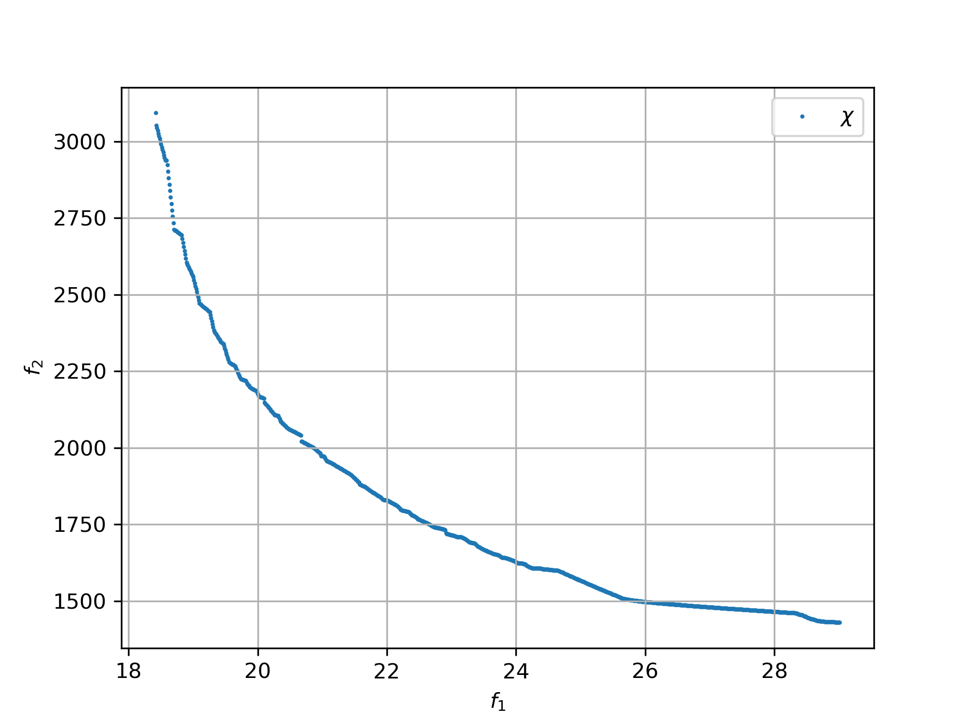

Only by combining all three Pareto fronts can we offer our boss the full set of alternatives.

Conclusion

Be careful with approximate models. They may oversimplify the problem, as our first Cassini model without deep-space maneuvers did.
Use a single objective algorithm to check what is possible.
Be careful when one objective is hard to compute and another can be derived directly from the decision variables.
Sometimes you need to combine solutions (Pareto fronts) from different methods to get a more complete multi-objective result.