fcmaes - a Python 3 gradient-free optimization library

How to use fcmaes

This tutorial uses a real-world example from space mission design. The repository also contains examples from mechanical component design and an example of optimization with ODEs in the objective function in ODE.

fcmaes makes several real-world space trajectory design tasks callable from Python:

Cassini1, Cassini2, Rosetta, GTOC1, Messenger reduced, Messenger full, Sagas, and Tandem

The original source code is available in GTOPToolbox. fcmaes adds a Python interface in astro.py. The code used in this tutorial is in tutorial.py. We focus on GTOC1 and leave the other problems for you to explore.

GTOC1

Assume we are taking part in the GTOC1 competition. The original task is a complex space mission problem: save Earth from an incoming asteroid impact. To optimize it, we first need an abstraction that is simpler but still useful as a basis for a full solution.

ESA provides such an abstraction here ESA-Abstraction, with an implementation in GTOPToolbox. If we could solve this abstraction well, it would already place us at rank 3 in the official (GTOC1-results).

The ESA-Abstraction fixes the planet sequence and replaces the ion thruster with a regular impulse engine. The cost function is available as astro.gtoc1Func. It takes an argument vector X and returns a double value. The function is only partly defined, but the given bounds ensure that we get a valid result. That value is the competition score. It combines several objectives through a weighted sum. The maximal thrust constraint is handled indirectly: a good score means that only "small" impulse maneuvers are needed, and these can be converted into a low-thrust trajectory.

Recommended way to solve GTOC1

We start with the recommended way to use fcmaes:

import math
import time
from fcmaes.optimizer import dtime
from fcmaes import astro, advretry

def test_advretry(problem, num):
    best = math.inf
    t0 = time.perf_counter();
    for i in range(num):
        ret = advretry.minimize(problem.fun, bounds = problem.bounds, num_retries = 4000)
        best = min(ret.fun, best)
        print("{0}: time = {1:.1f} best = {2:.1f} f(xmin) = {3:.1f}"
              .format(i+1, dtime(t0), best, ret.fun))

if __name__ == '__main__':
	problem = astro.Gtoc1()
	test_advretry(problem, 10)

We run 10 experiments with 4000 retries each. All other parameters stay at their defaults. On a 16-core AMD 3950x, the output looks like this:

1: time = 89.2 best = -1581950.2 f(xmin) = -1581950.2
2: time = 177.6 best = -1581950.3 f(xmin) = -1581950.3
3: time = 267.4 best = -1581950.3 f(xmin) = -1581950.3
4: time = 356.3 best = -1581950.3 f(xmin) = -1581950.3
5: time = 445.0 best = -1581950.3 f(xmin) = -1581950.3
6: time = 534.5 best = -1581950.3 f(xmin) = -1581950.2
7: time = 623.5 best = -1581950.3 f(xmin) = -1581950.3
8: time = 712.5 best = -1581950.3 f(xmin) = -1581950.3
9: time = 799.9 best = -1581950.3 f(xmin) = -1581950.3
10: time = 887.7 best = -1581950.3 f(xmin) = -1567308.5

In 9 out of 10 runs we reach the optimum. Each run takes about 90 seconds. So why spend time on such an "easy" problem? At the actual GTOC1 competition, most teams scored lower. fcmaes hides much of the difficulty of this benchmark. To see that more clearly, we now try several alternative methods on the GTOC1 problem.

Coordinated Retry using CMA-ES

Using the optimizer parameter of advretry.minimize, we can replace the default optimizer. Let us try CMA-ES:

from fcmaes.optimizer import Cma_python, dtime
...
        ret = advretry.minimize(problem.fun, bounds = problem.bounds, num_retries = 4000,
                   optimizer = Cma_python(2000))
...

The parameter passed to Cma_python(2000) is the initial maximum number of function evaluations per optimization run. Coordinated retry increases this limit every 100 runs. Starting with a low limit is useful because, early on, coordinated retry does not yet know where to focus the search and should not spend too many evaluations at once. fcmaes.optimizer also lets you build optimizers as sequences of other optimizers. In that case, the evaluation budget can be split across the sequence members, and advretry.minimize increases their limits proportionally. Here we get:

1: time = 118.2 best = -1559737.6 f(xmin) = -1559737.6
2: time = 232.0 best = -1570386.7 f(xmin) = -1570386.7
3: time = 348.5 best = -1570386.7 f(xmin) = -1568160.4
4: time = 464.0 best = -1570386.7 f(xmin) = -1565316.2
5: time = 577.6 best = -1581950.2 f(xmin) = -1581950.2
6: time = 692.8 best = -1581950.2 f(xmin) = -1570386.7
7: time = 809.8 best = -1581950.2 f(xmin) = -1567308.4
8: time = 924.9 best = -1581950.2 f(xmin) = -1577088.6
9: time = 1037.8 best = -1581950.2 f(xmin) = -1581950.2
10: time = 1152.2 best = -1581950.2 f(xmin) = -1581950.2

CMA-ES was the default optimizer in earlier versions of fcmaes. This result shows why it was replaced by a DE→CMA sequence. The performance is still reasonable, but we get only three hits out of ten. It is also slower, although Cma_cpp(2000), the C++ variant, can reduce that cost.

Parallel Retry

Simple parallel retry is sometimes the better choice, especially for high-dimensional problems or expensive objective functions.

from fcmaes import astro, retry
...
        ret = retry.minimize(problem.fun, bounds = problem.bounds,
                num_retries = 2000, max_evaluations = 100000)
...

Here we raise the fixed evaluation limit to 100000. This shows that even with a larger budget than the advretry.minimize default of 50000 evaluations, results on GTOC1 are worse:

1: time = 72.0 best = -1394701.3 f(xmin) = -1394701.3
2: time = 143.9 best = -1394701.3 f(xmin) = -1349303.4
3: time = 215.4 best = -1448108.2 f(xmin) = -1448108.2
4: time = 287.2 best = -1508157.0 f(xmin) = -1508157.0
5: time = 359.1 best = -1513210.8 f(xmin) = -1513210.8
6: time = 430.6 best = -1513210.8 f(xmin) = -1489635.2
7: time = 502.0 best = -1513210.8 f(xmin) = -1506445.5
8: time = 573.6 best = -1523622.8 f(xmin) = -1523622.8
9: time = 645.2 best = -1523622.8 f(xmin) = -1503193.3
10: time = 716.8 best = -1523622.8 f(xmin) = -1519143.8

Parallel Retry using CMA-ES

...
        ret = retry.minimize(problem.fun, bounds = problem.bounds,
                num_retries = 2000, optimizer = Cma_python(100000))
...

This time we must pass the evaluation limit to Cma_python(100000), just as we did for coordinated retry. Simple retry does not increase this limit on its own.

1: time = 78.1 best = -1404487.1 f(xmin) = -1404487.1
2: time = 154.2 best = -1404487.1 f(xmin) = -1392344.8
3: time = 230.4 best = -1503193.1 f(xmin) = -1503193.1
4: time = 307.9 best = -1503193.1 f(xmin) = -1425075.5
5: time = 385.7 best = -1503193.1 f(xmin) = -1399988.7
6: time = 463.0 best = -1542602.2 f(xmin) = -1542602.2
7: time = 540.3 best = -1579084.3 f(xmin) = -1579084.3
8: time = 618.0 best = -1579084.3 f(xmin) = -1395664.8
9: time = 697.0 best = -1579084.3 f(xmin) = -1395664.9
10: time = 775.3 best = -1579084.3 f(xmin) = -1426918.2

Without coordinated retry, CMA-ES can still compete with the default optimizer.

Logging

You can enable logging, including for advretry.minimize, like this:

from fcmaes.optimizer import logger
...
        ret = retry.minimize(problem.fun, bounds = problem.bounds, num_retries = 4000,
                   logger = logger())
...

Logging writes both to the screen and to a log file. The Readme describes the log output in more detail. Mean values and standard deviations across runs are useful when comparing optimization algorithms.

...
8.41 1303740 256 10964457 -1512825.931527 -654747.84 297959.56 [-1475105.69, -1306121.73, -1250238.61,

This line means that after 8.41 seconds we had 256 runs, 10964457 evaluations, and 1303740 evaluations per second. The best result was -1512825, with mean = -654747 and sdev = 297959. We also see the best 20 results, followed by the best solution so far. For advretry.minimize, the output differs slightly because a varying number of function evaluations makes mean and sdev less meaningful.

Serial Loop using CMA Python

Next, let us see what happens when we replace parallel retry with a simple loop:

from fcmaes import cmaes
...
    best = math.inf
    t0 = time.perf_counter();
    for i in range(1000):
        ret = cmaes.minimize(problem.fun, max_evaluations = 100000, bounds = problem.bounds)
        if best > ret.fun or i % 100 == 99:
            print("{0}: time = {1:.1f} best = {2:.1f} f(xmin) = {3:.1f}"
              .format(i+1, dtime(t0), best, ret.fun))
        best = min(ret.fun, best)

We get:

1: time = 0.8 best = inf f(xmin) = -84473.9
3: time = 2.2 best = -84473.9 f(xmin) = -685008.5
4: time = 3.0 best = -685008.5 f(xmin) = -696421.2
5: time = 3.7 best = -696421.2 f(xmin) = -864561.8
22: time = 18.3 best = -864561.8 f(xmin) = -1136598.3
52: time = 43.3 best = -1136598.3 f(xmin) = -1227708.5
100: time = 83.8 best = -1227708.5 f(xmin) = -1166085.7
200: time = 167.8 best = -1227708.5 f(xmin) = -942740.5
265: time = 220.8 best = -1227708.5 f(xmin) = -1415819.8
300: time = 248.3 best = -1415819.8 f(xmin) = -43348.4
317: time = 262.7 best = -1415819.8 f(xmin) = -1467685.3
400: time = 330.2 best = -1467685.3 f(xmin) = -1109849.9
500: time = 407.1 best = -1467685.3 f(xmin) = -73631.4
600: time = 487.4 best = -1467685.3 f(xmin) = -833640.3
700: time = 573.9 best = -1467685.3 f(xmin) = -411707.5
800: time = 656.1 best = -1467685.3 f(xmin) = -316534.2
900: time = 737.3 best = -1467685.3 f(xmin) = -69421.9
1000: time = 818.2 best = -1467685.3 f(xmin) = -545722.6

For 1000 retries, we need 818 seconds and get a decent result of -1467685.

Serial Loop using CMA C++

The Python CMA implementation can be replaced easily with the C++ version:

from fcmaes import cmaescpp
...
    best = math.inf
    t0 = time.perf_counter();
    for i in range(1000):
        ret = cmaescpp.minimize(problem.fun, max_evaluations = 100000, bounds = problem.bounds)
        if best > ret.fun or i % 100 == 99:
            print("{0}: time = {1:.1f} best = {2:.1f} f(xmin) = {3:.1f}"
              .format(i+1, dtime(t0), best, ret.fun))
        best = min(ret.fun, best)

We get:

1: time = 1.1 best = inf f(xmin) = -83800.5
4: time = 2.6 best = -83800.5 f(xmin) = -1415819.7
100: time = 52.0 best = -1415819.7 f(xmin) = -787091.1
200: time = 101.1 best = -1415819.7 f(xmin) = -63063.6
300: time = 151.4 best = -1415819.7 f(xmin) = -76361.4
327: time = 164.9 best = -1415819.7 f(xmin) = -1512825.9
400: time = 201.4 best = -1512825.9 f(xmin) = -423970.3
500: time = 251.1 best = -1512825.9 f(xmin) = -602149.4
600: time = 300.2 best = -1512825.9 f(xmin) = -565361.7
700: time = 349.8 best = -1512825.9 f(xmin) = -589410.0
800: time = 399.7 best = -1512825.9 f(xmin) = -73190.7
900: time = 448.1 best = -1512825.9 f(xmin) = -76455.3
1000: time = 499.1 best = -1512825.9 f(xmin) = -64913.0

The speed difference compared to the Python variant is surprisingly small. If you have worked with other Python CMA implementations, you might expect a larger gap.

The Ask / Tell interface

The ask / tell interface gives the calling code full control over the evaluation process. Some optimization frameworks, such as nevergrad, require this interface for all optimization algorithms they use, including fcmaes.cmaes.

from fcmaes import cmaes
...

    best = math.inf
    t0 = time.perf_counter();
    for i in range(num):
        es = cmaes.Cmaes(bounds = problem.bounds)
        iters = 3000
        for j in range(iters):
            xs = es.ask()
            ys = [problem.fun(x) for x in xs]
            stop = es.tell(ys)
            if stop != 0:
                break
        best = min(es.best_value, best)
        print("{0}: time = {1:.1f} best = {2:.1f} f(xmin) = {3:.1f}"
              .format(i+1, dtime(t0), best, es.best_value))

Results in:

1: time = 0.8 best = -29735.1 f(xmin) = -29735.1
2: time = 1.5 best = -433772.0 f(xmin) = -433772.0
3: time = 2.5 best = -559867.7 f(xmin) = -559867.7
4: time = 3.5 best = -1230104.7 f(xmin) = -1230104.7
...

Parallel Objective Function Evaluation

For GTOC1 this does not help much, but for very expensive objective functions it can be better to skip parallel retry and instead evaluate the objective in parallel within a single optimization run. nevergrad supports this more generally. In fcmaes, only the Python variant of CMA-ES supports it:

from fcmaes import cmaes
...
    best = math.inf
    t0 = time.perf_counter();
    for i in range(1000):
        ret = cmaes.minimize(problem.fun, bounds = problem.bounds, workers = mp.cpu_count())
        if best > ret.fun or i % 100 == 99:
            print("{0}: time = {1:.1f} best = {2:.1f} f(xmin) = {3:.1f}"
              .format(i+1, dtime(t0), best, ret.fun))
        best = min(ret.fun, best)

We get:

1: time = 1.3 best = inf f(xmin) = -68805.8
2: time = 2.1 best = -68805.8 f(xmin) = -1234368.5
100: time = 111.7 best = -1234368.5 f(xmin) = -51568.7
159: time = 172.9 best = -1234368.5 f(xmin) = -1262436.0
200: time = 218.9 best = -1262436.0 f(xmin) = -494445.5
284: time = 304.6 best = -1262436.0 f(xmin) = -1307412.3
300: time = 321.6 best = -1307412.3 f(xmin) = -43115.4
...

We do not see any speedup compared to serial execution. Python multiprocessing must be used carefully. For GTOC1, the overhead of parallelizing objective calls can outweigh the benefit, especially on Windows. Use this only when function evaluations are truly expensive, more than 0.1 seconds. Otherwise, use parallel or coordinated retry to use all CPU cores more effectively.

Serial Loop using Scipy Differential Evolution

If you are using SciPy, Differential Evolution is probably the best option for GTOC1. We do not limit the number of evaluations so it gets a fair chance.

from scipy.optimize import differential_evolution
...
    best = math.inf
    t0 = time.perf_counter();
    for i in range(num):
        ret = differential_evolution(problem.fun, bounds = problem.bounds)
        if best > ret.fun or i % 100 == 99:
            print("{0}: time = {1:.1f} best = {2:.1f} f(xmin) = {3:.1f}"
              .format(i+1, dtime(t0), best, ret.fun))
        best = min(ret.fun, best)

We get:

1: time = 7.2 best = inf f(xmin) = -1199635.8
16: time = 107.4 best = -1199635.8 f(xmin) = -1203199.8
28: time = 190.2 best = -1203199.8 f(xmin) = -1314267.1
100: time = 678.1 best = -1314267.1 f(xmin) = -815122.2
169: time = 1148.7 best = -1314267.1 f(xmin) = -1458167.2
200: time = 1360.6 best = -1458167.2 f(xmin) = -1268824.3
240: time = 1639.1 best = -1458167.2 f(xmin) = -1540128.6
300: time = 2054.4 best = -1540128.6 f(xmin) = -955791.7
400: time = 2749.1 best = -1540128.6 f(xmin) = -708363.0
500: time = 3433.1 best = -1540128.6 f(xmin) = -762684.0
600: time = 4121.4 best = -1540128.6 f(xmin) = -489924.5
700: time = 4795.7 best = -1540128.6 f(xmin) = -1102244.1
800: time = 5468.0 best = -1540128.6 f(xmin) = -1003071.6
900: time = 6154.7 best = -1540128.6 f(xmin) = -623171.3
1000: time = 6846.3 best = -1540128.6 f(xmin) = -1229926.1

That is almost two hours for 1000 runs, with a decent but not optimal result. SciPy Differential Evolution differs from the fcmaes implementation and does not solve GTOC1 in a reasonable time.

Serial Loop using Scipy Dual Annealing

Dual Annealing is the second SciPy algorithm that can be recommended for GTOC1:

from scipy.optimize import dual_annealing
...
    best = math.inf
    lb = problem.bounds.lb
    ub = problem.bounds.ub
    t0 = time.perf_counter();
    for i in range(num):
        ret = dual_annealing(problem.fun, bounds = list(zip(lb, ub)))
        if best > ret.fun or i % 100 == 99:
            print("{0}: time = {1:.1f} best = {2:.1f} f(xmin) = {3:.1f}"
              .format(i+1, dtime(t0), best, ret.fun))
        best = min(ret.fun, best)

We get:

1: time = 1.5 best = inf f(xmin) = -478299.5
2: time = 3.9 best = -478299.5 f(xmin) = -1037793.1
25: time = 58.6 best = -1037793.1 f(xmin) = -1153125.0
100: time = 226.7 best = -1153125.0 f(xmin) = -59482.4
195: time = 449.4 best = -1153125.0 f(xmin) = -1316793.6
200: time = 460.0 best = -1316793.6 f(xmin) = -481995.4
300: time = 689.6 best = -1316793.6 f(xmin) = -33647.2
400: time = 930.7 best = -1316793.6 f(xmin) = -63162.0
500: time = 1170.7 best = -1316793.6 f(xmin) = -47384.3
600: time = 1407.1 best = -1316793.6 f(xmin) = -40991.5
632: time = 1483.0 best = -1316793.6 f(xmin) = -1537477.6
700: time = 1641.9 best = -1537477.6 f(xmin) = -227272.4
800: time = 1885.2 best = -1537477.6 f(xmin) = -71036.6
900: time = 2115.2 best = -1537477.6 f(xmin) = -374102.7
1000: time = 2348.6 best = -1537477.6 f(xmin) = -537919.7

This is faster than SciPy Differential Evolution and gives a similar result.

Serial Loop using Scipy minimize

scipy.optimize.minimize is meant for local optimization, but it is fast. What happens if we run 200000 retries?

from scipy.optimize import minimize
...
    best = math.inf
    t0 = time.perf_counter();
    for i in range(num):
        guess = random_x(problem.bounds.lb, problem.bounds.ub)
        ret = minimize(problem.fun, x0 = guess, bounds = problem.bounds)
        if best > ret.fun or i % 20000 == 19999:
            print("{0}: time = {1:.1f} best = {2:.1f} f(xmin) = {3:.1f}"
              .format(i+1, dtime(t0), best, ret.fun))
        best = min(ret.fun, best)

We get:

1: time = 0.0 best = inf f(xmin) = -66.1
5: time = 0.1 best = -66.1 f(xmin) = -144.6
6: time = 0.1 best = -144.6 f(xmin) = -1439.1
15: time = 0.2 best = -1439.1 f(xmin) = -30308.5
37: time = 0.4 best = -30308.5 f(xmin) = -35758.5
340: time = 4.0 best = -35758.5 f(xmin) = -46205.2
846: time = 11.1 best = -46205.2 f(xmin) = -258336.1
2293: time = 30.2 best = -258336.1 f(xmin) = -603667.3
20000: time = 271.5 best = -603667.3 f(xmin) = -0.2
40000: time = 545.3 best = -603667.3 f(xmin) = -0.0
60000: time = 823.7 best = -603667.3 f(xmin) = -0.0
80000: time = 1097.1 best = -603667.3 f(xmin) = -448.5
100000: time = 1367.1 best = -603667.3 f(xmin) = -0.0
120000: time = 1647.0 best = -603667.3 f(xmin) = -75.0
130210: time = 1786.9 best = -603667.3 f(xmin) = -637330.4
140000: time = 1918.2 best = -637330.4 f(xmin) = -0.0
160000: time = 2187.6 best = -637330.4 f(xmin) = -0.0
180000: time = 2459.2 best = -637330.4 f(xmin) = -8.1
181671: time = 2481.2 best = -637330.4 f(xmin) = -687313.0
200000: time = 2728.2 best = -687313.0 f(xmin) = -1952.0

Even with 200000 retries, a local optimizer still gives a poor best result on GTOC1. That is not surprising, but it does show that GTOC1 is far less trivial than it first appeared.

Winning the GTOC1 Competition

GTOC1 was the first in a series of interesting space trajectory optimization competitions. For years, it was almost impossible to beat both ESA and JPL, which is not surprising given that they were the two strongest participants overall. GTOC1 was organized by ESA and won by JPL with an almost perfect solution. With the ESA abstraction, we cannot reach JPL’s winning score of -1850000. Adding more planets to the trajectory helps, but there is another issue:

The number of revolutions around the sun is chosen from the minimal deltaV at departure from a planet. Higher deltaV means we need more fuel. This choice determines the incoming arc at the next planet, so a locally good decision can turn out to be poor for the full trajectory. To find the optimum, we have to branch over the number of revolutions for each planet-to-planet transfer.

Note	The original `revolutions.png` search-tree figure is not present in this repository.

We chose the following planet sequence: EVVEVVEESJA (E = Earth, V = Venus, J = Jupiter, S = Saturn, A = incoming asteroid) With the old deterministic objective function, this gives an optimal score of around -1670000.

Replacing search by optimization

In most cases, the locally optimal number of revolutions is also globally optimal. We assign probabilities to the child nodes based on local deltaV. Low-deltaV branches get high probabilities. We then adapt the objective function so it chooses the number of revolutions according to those probabilities. This makes the objective noisy, or non-deterministic, but removes the need for an explicit search algorithm.

Now let us look at the results. This time we use a different processor, the 32-core AMD 2990WX. It is known to have scaling issues because of its internal design. Even so, coordinated parallel retry scales well on this processor, as the results show:

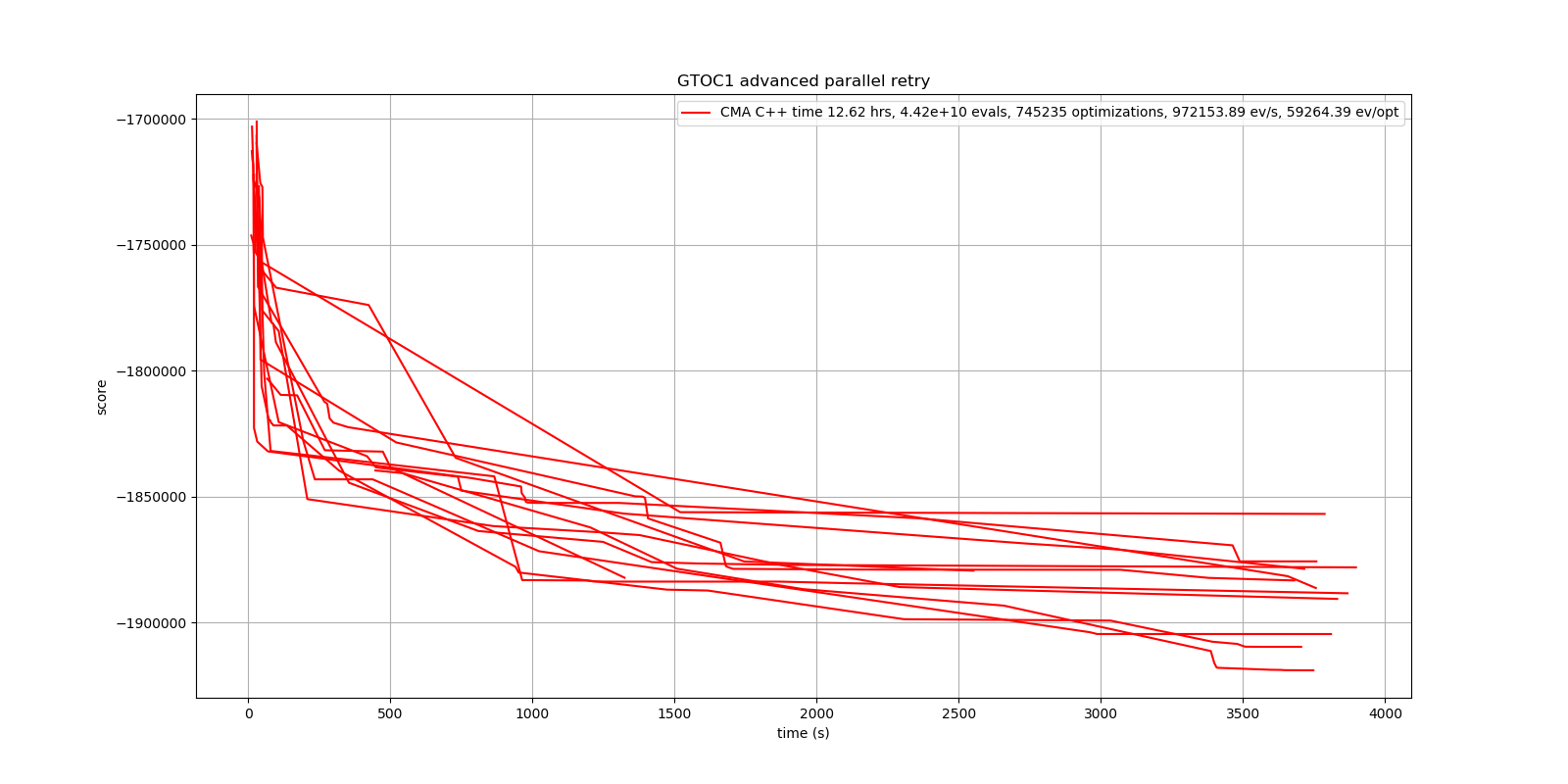
The best solution scores around -1920000. Objective function evaluation takes a bit longer because we now have ten planet-to-planet transfers. We get 970000 evaluations / sec, compared to around 600000 on the AMD 3950x used earlier. To compute a real GTOC1 solution, this impulse-based trajectory still has to be converted into a low-thrust trajectory. Here is a video of a GTOC1 solution using the EVVEVVEESJA sequence that I computed in 2018 with this method.