fcmaes - a Python 3 gradient-free optimization library

Quality-Diversity applied to ODE based control problems

This tutorial

Discusses how to apply QD-algorithms (Quality Diversity) to ODE based control problems.
Discusses the history of solving optimization problems involving integrals and control.
Compares the analytical approach with a "smart guessing with feedback" approach on a simple example: dampening a spring.

Learning from nature

Let us start with two important statements from Why Greatness Cannot Be Planned: The Myth of the Objective:

"Natural evolution can be seen as a novelty-generating search with local competition".
"Global competition naturally leads to convergence while local competition naturally enhances diversity and creativity."

The book argues that the competitive or "survival of the fittest" aspect of evolution is not what creates interesting results. Competition tends to reduce diversity. Other mechanisms, such as drift and exaptation, are more important here. Exaptation means that a mutation becomes useful later in a different and unexpected context.

Simulating this in an optimization algorithm costs resources. Local competition requires many niches to be represented and stored, which is what enables local competition and "creativity". Still, at a sufficient level of parallelism, the benefits can outweigh the cost. CPUs, GPUs, and TPUs keep adding more cores, and our algorithms should adapt to that.

History of the "smart guessing approach"

The "smart guessing" approach has existed for a long time. It gained real momentum with machine learning based on neural networks. Neural networks perform prediction or classification by analyzing input data and transforming it through several connected layers of artificial neurons. The weights of these connections are the decision variables of an optimization problem. The goal is to minimize prediction or classification error on test data.

Although this is sometimes described as alchemy, there is simply no analytical way to solve the optimization step. Instead, we start with an often random guess, evaluate the network, measure the error, and use that error as feedback to improve the guess in a loop.

Gradient-based methods dominated for a while. More recently, evolutionary methods have also been used, see EvoJAX. Neural networks were considered a dead end for several decades. That changed when modern GPUs and TPUs made it possible to process many thousands of neurons in parallel. How a method is perceived often depends on the hardware available at the time.

History of the analytical approach

Appendix 2 of DEANGELIS_FEDERICO presents a useful history of the analytical approach to optimization problems involving integrals and control, known as optimal control theory: "Optimal control theory can be conceived as the last step of a long journey, which started with geometrical problems of Ancient Greek philosophers, went through the 17th , 18th and 19th centuries when the Calculus of Variations (the “ancestor” of optimal control theory) was developed, ending with the fundamental contributions of Lev Pontryagin and Richard Bellman in the 1950s’". The researchers who developed the analytical approach over the centuries had very limited "hardware" available. It was reasonable for them to believe that their approach was the only practical way to solve these problems.

But, as machine learning has shown, that can change. Instead of evaluating a single integral, we can now compute billions of them in a few minutes on a modern many-core CPU. In this tutorial we will see that "smart guessing" can reproduce the analytical result in seconds. It can also reveal the structure of the problem in ways the analytical approach does not easily provide.

Dampening a Vibrating Spring

We use the example from EXAMPLE 2: CONTROL OF A VIBRATING SPRING, page 37.

x1(t) denotes the position over time t, x2(t), its derivative is the velocity.
The derivative of x2(t) is -x1(t) + alpha(t), which means the acceleration pushing the spring back in its original position grows with its extension. Additionally, we apply an additional "force" alpha(t), which is the "control" we have over the dynamic system.

The full example code is at damp.py and ascent.cpp.

If no external force is applied we get:

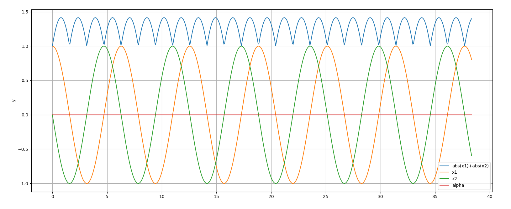
The blue line represents abs(x1) + abs(x2). This value is easy to measure. When it reaches 0, the spring is fully damped. We can drive it there by applying specific alpha values over time:

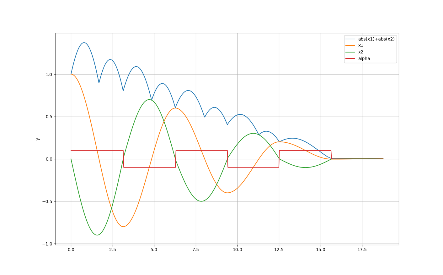
EXAMPLE 2 shows the analytical derivation of the optimal control. As in the figure above, the resulting control alpha switches exactly when the velocity x2 crosses 0. This type of control is called "bang bang".

Guessing with feedback

To implement the "guessing" approach, we first need a fast integrator: Ascent. The two differential equations are coded in C++:

struct Damp {

    double alpha;

    void operator()(const state_t &y, state_t &yDot, const double) {

        double x1 = y[0];
        double x2 = y[1];
        yDot[0] = x2;
        yDot[1] = -x1 + alpha;
    }
};

Next we create a function integrateDamp_C that can be called from Python via ctypes. It performs the integration in a loop. Since we use a fixed alpha, the function has to be called repeatedly, once for each time segment.

extern "C" {
double* integrateDamp_C(double *yd, double alpha, double dt, double step) {
    state_t y(2);
    for (int i = 0; i < 2; i++)
        y[i] = yd[i];
    PC233 integrator;
    Damp damp;
    damp.alpha = alpha;
    int steps = 0;
    double t = 0.0;
    while (t < dt) {
        steps++;
        if (t + step >= dt) {
            integrator(damp, y, t, dt - t);
            break;
        } else
            integrator(damp, y, t, step);
    }
    double *res = new double[2];
    for (int i = 0; i < 2; i++)
        res[i] = y[i];
    return res;
}

void free_mem(double *a) {
    delete[] a;
}

Writing this code is straightforward, even for much more complex ODE systems. For those systems, finding an analytical solution can be very hard. The following Python code calls the C++ function. To avoid a memory leak, we free the result vector after converting it to a numpy array. Be careful with all data structures created on the heap, such as double *res = new double[2].

def integrate_C(y, dt, alpha, step):
    array_type = ct.c_double * y.size
    ry = integrateDamp_C(array_type(*y), alpha, dt, step)
    y = np.array(np.fromiter(ry, dtype=np.float64, count=y.size))
    free_mem(ry)
    return y

It would be easier to use scipy.integrate.ode, but it is about a factor of 10 slower.

Next we define a single-objective fitness function. It calls integrate_C in a loop and applies different alpha values over different time intervals, all determined by the decision vector X. We add a penalty for max_time violations so the optimizer is forced to finish the dampening process in time. The number of decision variables self.dim determines the number of time intervals n = self.dim/2. We normalize the possible alpha values to the interval [-max_alpha, +max_alpha].

   def __call__(self, X):
        n = int(self.dim/2)
        dt = 2*max_time/n
        dts = X[:n]*dt
        alphas = X[n:]*2*max_alpha - max_alpha
        y = np.array([1,0])
        for i in range(n):
            y = integrate_C(y, dts[i], alphas[i], 0.1)
        y = abs(y[0])+abs(y[1])
        t = sum(dts)
        if t > max_time: # penalty for not finishing in time
            y += 100 + t
        return y

A single-objective optimizer, for example parallel retry of differential evolution, can solve the problem in less than a second:

def parallel_retry(dim, opt = De_cpp(10000)):
    fit = fitness(dim)
    return retry.minimize(fit, fit.bounds, optimizer=opt, num_retries=32)

How does differential evolution work? It starts with random values for the time intervals and the alpha values used in them. As feedback, it receives abs(x1) + abs(x2), our approximation of the final amplitude. Based on that value, it generates new random values. This makes it a typical example of the "smart guessing" approach.

But recall the discussion about natural evolution. Natural evolution is a novelty-generating search with local competition. Differential evolution uses global competition, so it tends to lose diversity and creativity. That is why we now investigate a QD (Quality-Diversity) algorithm, which is closer to natural evolution because it creates niches and supports local evolution.

Applying MAP-Elites

First we create a QD-fitness function qd_fit. It uses call, but also returns a behavior or feature vector b containing the overall time np.sum(dts) and the energy consumption np.sum(np.multiply(dts, abs(alphas))). This lets us distinguish solutions by time and energy.

    def qd_fit(self, x):
        y = self(x)
        n = int(self.dim/2)
        dt = 2*max_time/n
        dts = x[:n]*dt
        alphas = x[n:]*2*max_alpha - max_alpha
        dtsum = np.sum(dts)
        energy = np.sum(np.multiply(dts, abs(alphas)))
        b = np.array([dtsum, energy])
        return y, b

As the QD algorithm we use diversifier. It normally runs MAP-Elites and an improvement emitter, usually based on CR-FM-NES, in parallel. That is a good default and often a good place to start. Here, however, experiments showed that it is better to skip the improvement emitter and run only MAP-Elites. So we dedicate all parallel processes to MAP-Elites and limit the number of fitness evaluations to 30 million. This means several hundred million integrations, which can be executed in about two minutes on an AMD 5950x 16 core CPU.

Note that this example requires fcmaes version 1.5.6. On the same hardware it is more than a factor of 2 slower on Windows. It is better to use the Linux subsystem for Windows. Python multiprocessing is still poorly implemented on Windows.

def optimize_qd(dim):
    problem = fitness(dim)
    name = 'damp_nd'
    opt_params0 = {'solver':'elites', 'popsize':512}
    archive = diversifier.minimize(
         mapelites.wrapper(problem.qd_fit, problem.qd_dim, interval=200000),
         problem.bounds, problem.qd_bounds, opt_params=[opt_params0], max_evals=30000000)
    print('final archive:', archive.info())
    archive.save(name)

Below are results for dim=8 (4 time intervals, left diagram) and dim=12 (6 time intervals, right diagram).

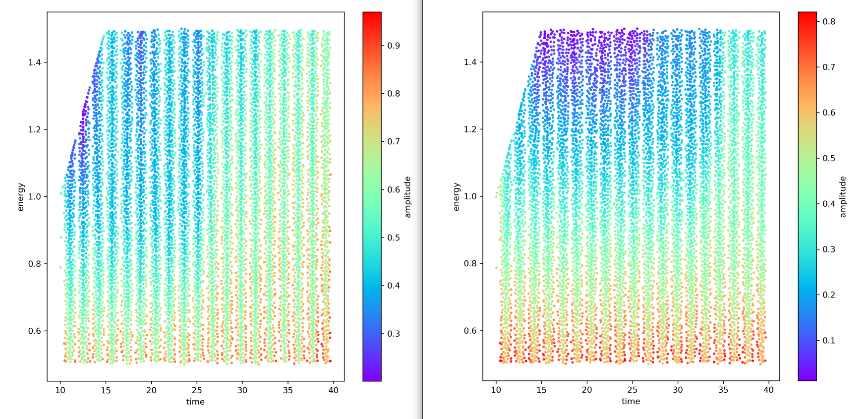
Four time intervals are not sufficient for complete dampening. For each overall time and energy value, we can see exactly which level of dampening is achievable. Each of the many thousand dots in both diagrams represents one solution stored in the QD archive file. This kind of insight into what is possible for different energy and time values is hard to reproduce with the analytical approach.

Conclusion

There is not much literature on applying QD methods to problems involving integrals and control, so there is little to compare against. The results here are therefore preliminary. Still, they can serve as a baseline for future comparisons.

Application of Ascent is easy and can result in a factor 10 speedup compared to scipy.integrate.ode.
MAP-Elites is not only able to provide insight into the structure of the problem, it can also find the global optimum in a reasonable amount of time, if all CPU-cores of a modern many-core CPU are utilized.
This cannot easily be achieved by the analytical approach.